Air Quality in the Barnett Shale - Part 20: Dr. Sattler's Deposition - The Gaussian Model

Well I thought I was done with this topic...but something occurred to me when I was reviewing a presentation on air dispersion modeling a friend of mine gave me.  Let me be clear on this up front.  I don't know nothin' about air dispersion modeling.  Math makes my head hurt.  However, I can sometimes look at something complex and get some semblance of understanding.

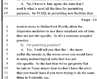
So Dr. Sattler in her Deposition stated that the air dispersion program was based on a Gaussian dispersion model:

What that means, is that the plume of chemicals (the smoke so-to-speak) coming from the end of the pipe (the smoke stack) behaves in a Gaussian manner:

In other words, if the wind direction stays constant, and the emission rates stays constant, and all the other atmospheric conditions stay constant, we can estimate the concentration at some point away from the stack:

This is based on the formula - what Dr. Sattler states is the "heart of the computer software" - which looks like this:

Because the samples were taken at "ground level" we use the formula to calculate a "ground level" concentration:

Does your head hurt yet?  Mine does....but bear with me.

So, for example under "normal" atmospheric conditions, this particular plume - over time - would look like this:

...and under "unstable" conditions we would expect it to look like this"

What this shows is...that with a smoke stack that is 25 meters high, a wind speed of 1 meter per second, and an emission rate coming out of the smoke stack of 1 gram of chemical per second, we would expect some concentration near what is modeled at some distance away from the stack in the "x" direction and some distance away in the "y" direction.  The wind direction stays constant - that's the center line - and x and y are some point around that center line line.

So if I know the stack hight, the wind speed, and the emission rate, and I know the atmospheric conditions, the concentration "C" at x and y distance at 0 - or ground "z" - can be estimated.

That's what Dr. Sattler did for Alisa Rich, only she did with 8760 hours of meteorological data provided to her:

But first she needed to calculate the emission rate "E."  And that's when it hit me...

To "back in" the concentration C(x,y,z) to get E, certain parameters needed to be fixed.  Dr. Sattler could estimate the stack hight "H," and she knew the canister was collected at ground level, so z = 0.  She also had the atmospheric conditions and wind speed for the 24 hours of the time the sample was collected.

And here is where I started to see a problem.  She has a sample that is fixed - it stayed in one spot and collected a sample over 24 hours.  The dispersion model tells you what the concentration will be at some distance away from the stack, that is, if I grab a sample at an x-y coordinate, I would would expect a concentration of C.  But the samples in which the the data on concentration was obtained to "back in" was many grab samples all collected and added together.

What's the problem with that?  Well in order for the Gaussian model to work, it assumes a center line:

So at an emission rate "E" of, lets say, 1 gram per second, and a wind speed "U" of 1 meter per second, at 10 meters in the direction of that center line, 10 grams have been released, with the concentration highest at the stack.  Now as the atmospheric conditions change - stable - unstable - how far that plume is dispersed will vary (see the two example above).

What this means...is in order for Dr. Sattler to "back in the concentration, she had to fix the wind direction (the center line).  So based on the wind direction chosen, the variable "y" can be determined.  But what concentration do you use for that x-y position?  Because the x-y concentration at a fixed z = 0, is a matter of wind speed and emission rate.  Since we know the wind speed, did she assume the total concentration collected over 24 hours was what determined that emission rate?

In other words, to get the benzene concentration of canister 4 (Table 1) that was located x and y distance from the source, with a known wind speed of "U", the emission rate "E" would be artificially high if it was backed in, since in the model, at x-y distance at wind speed "U" and emission rate "E", the concentration "C" is predicted to be at some value.  

Since we know that value "C" and we know the wind speed "U", and we know the x-y coordinates of the sample canister, I am wondering if she set "E" based on the 24 hour concentration?  If that's how she did it, then "E" in all other model days would be extremely inflated.  It is possible that she compensated for this by knowing how much time elapsed based on the wind speed to get from the source to the canister - and then divided the 24 hour concentration by that time frame to get an average.

But even if that was done, there is another problem with her premise of "backed in" data and the Gaussian model's assumptions...

My head really hurts now....

Next post: Air Quality in the Barnett Shale - Part 21: Dr. Sattler's Deposition - If you assume E to be...

.