Air Quality in the Barnett Shale - Part 23: Fort Worth League of Neighborhoods Report to FWISD

I received a PDF of a photocopy of a report, dated February 2011, dealing with "Recommendations for Policy Changes for Gas Drilling Near Schools."

As you can see, it brings forth a concern regarding carbon disulfide and uses language that completely disregards the concept of dose, which if you have been reading all 20-something of these posts, was the original issue that started me on this topic.

Okay...so again with the carbon disulfide!  What does this report have to say about that chemical?  Reading... reading.... oh...you have got to be kidding me.  Well no wonder! Seems the same sampling method, the same analytical method, the same premise, the same model assumptions, the same poor science was involved in putting this report together.

It's Dr. Sattler's modeling work!  The same methodology and the same premise was used to produce these setback findings as was performed previously for Alisa Rich.  The same faulty logic that she was raked over the coals for in her December Deposition.  The same methodology I have been writing about in this blog as a way to explain why it is not just wrong, but demonstrably wrong.

I have whipped that dispersion model horse enough, as well as TICs, dose, sample size, and everything else that factors into why her premise and its resulting data are wrong, so I will focus on another factor that really needs to be considered when looking at her work and the conclusion she allows to be made.

What really aggravates me about this is that she knows her work does not meet intellectually honest or scientifically sound practices.  She was told this by the lawyer in the Deposition.  Even if she disagreed, the prudent thing to have done was double checked his concerns.  That obviously did not take place.
And now she not only puts her stamp of approval on it, she brings in another academic, Dr. David Sterling, Chair of Environmental and Occupational Health at the University of North Texas, Health Science Center.  And with him on board, her work, her model's predictions, this report's conclusion, is given the seal of scientifically soundness and approval:

These professionals agreed to assess the information available and make recommendations to the FWISD which could be incorporated into future leases.

This means that all three of them looked at her work and saw nothing wrong with it.  How can this be?

Okay, so lets look at it strictly from a logical point of view.  Let's assume that her model is correct - that every reason I have wrote about is immaterial or does not apply.  So logically if the following is true:

And the model predicted:

This would mean that the emission rate from the source - an emission rate that remains constant for 8760 hours - must be producing way in excess of 241 mg/m3 if that amount was found at up to one mile from the source.

Now according to the model, under calm conditions - perfect so to speak - the concentration at 1000 meters from the stack right smack dab down the center, is 0.001 g/m3 at 1 g/s.  So using that same ratio of dilution, the stack would be putting out at least 241000 mg/s or 241 grams/s of carbon disulfide.

That's a heck of a lot of carbon disulfide in and around the stack.  In fact, to get that much carbon disulfide at one mile from the stack, the amount of carbon disulfide in the immediate area would be at a lethal concentration.

Here is what ATSDR has to say about carbon disulfide (241 mg/m3 = 78 ppm):

• OSHA PEL (permissible exposure limit) = 20 ppm (averaged over an8-hour work shift); 30 ppm (acceptable ceiling concentration; 100 ppm (30-minute maximum peak)
• NIOSH IDLH (immediately dangerous to life or health) = 500 ppm
• AIHA ERPG-2 (maximum airborne concentration below which it is believed that nearly all persons could be exposed for up to 1 hour without experiencing or developing irreversible or other serious health effects or symptoms that could impair their abilities to take protective action) = 50 ppm
• Inhalation is the major route of exposure to carbon disulfide. The vapors are readily absorbed by the lungs. The odor threshold is approximately 200 to 1,000 times lower than the OSHA PEL-TWA (20 ppm). Odors of pure or commercial grades of carbon disulfide usually provide adequate warning of hazardous concentrations

So what this is saying - and here is where the logic comes in - If the one mile concentration could get up to as high as 78 ppm, the emission rate "E" necessary to produce that potential concentration at that distance must be considerably above 78 ppm.  If the model she predicted 241 mg/m3 is true, then the consistent output at the stack must be far greater than 78 ppm.  Which means that whenever the source is in operation, more than 78 ppm of carbon disulfide is being put into the air.

So if the model she predicts 241 mg/m3 is true, the output - "E" - must be producing carbon disulfide in abundance in order to push that much carbon disulfide down the plume to a distance of one mile.

And if that were true, people living in and around these sites at less than1000 meters would be constantly smelling an odor, and - most significantly - these oil & gas production sites would have a lot of very sick or dead workers.

And that is just not happening.  Do people complain about odors?  Yes, but at Dr. Sattler's calculated emission rate, the smell would be constant and never ending since the odor threshold is between  0.1 and 0.2 ppm. And if the level at one mile is 3 times the PEL, the workers at the source would be experiencing consistent health related problems.

This is not happening because there IS NO carbon disulfide being produced at these sites above an amount that will exceed an ESL, cause long or short term harm, or produce an odor.  Not at one mile nor next to the site.  None...at any distance around the facility.

So once again, to show why:

• Dr. Sattler's premise that you can "back in" a concentration to obtain the emission rate "E" is wrong.
• Dr. Sattler's positive identification of carbon disulfide - using EPA Method TO14 - is wrong.
• Dr. Sattler's quantification of carbon disulfide - identified by the lab as a TIC - is wrong.

And because these three things are wrong, her model's predictions are wrong - not off by a little - but wrong.

And because her model's predictions are wrong, the conclusion of the report - based on carbon disulfide concentrations - is wrong.

Next post: Air Quality in the Barnett Shale - Part 24: How confident in that 33.6 ug/m3 are you?

.

Air Quality in the Barnett Shale - Part 22: Gaussian for one, Gaussian for all

I was driving home from San Antonio so I had a lot of "me" time in the car.  Instead of thinking about non-work related stuff, my brain got busy thinking about the air dispersion model used for the Town of Dish, Texas, and for the "Fort Worth League of Neighborhoods" in their report to the Fort Worth Independent School District.

All of the modeling - modeling based on the science and math behind a Gaussian dispersion - is predicated on assumptions.  Not that there is anything wrong with that, it's just that if the assumption holds true in one part it must also hold true for the rest.

So my mind is mulling this over and over.  The math behind it is daunting, especially for a guy like me, but the premise, now that is something I think I do understand.

So in the Gaussian model, which is what Dr. Sattler uses, the premise is this:

If you know the wind direction, wind speed, stack height, atmospheric conditions, and emission rate, you can estimate the plume shape and concentration of the contaminant exiting the stack at any point within the plume.

It assumes that under fixed conditions for that run - fixed air speed, fixed emission rate, fixed atmospheric conditions, fixed exhaust stack height - the plume will behave in a Gaussian manner, that is, along a fixed center line (wind direction) the plume will behave the same on each side of that line.  What these models are used for is to say, that under the most ideal conditions it would be possible for a receptor so many meters away to be potentially exposed to this much of the contaminant at that stack height and that emission rate.

Since there is nothing we can do about the wind and weather, we can adjust the stack height or adjust the emission rate to decrease the intensity of the plume for that receptor.  The emission rate is often tweaked by adding pollution control devices on the stack or limiting the production the entity can produce.  No business likes to do less production so its mostly pollution control devices that are used - or sometimes - raising the height of the stack.

In order for Dr. Sattler to generate her models, she had to assume a fixed condition as well to plug into the computer model, a model that she says uses the Gaussian formula:

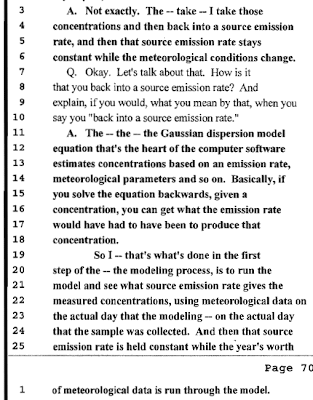
She had wind and atmospheric conditions for the day of sampling, so those could be plugged in.  She could reasonably estimate the stack hight for the compressors.  What she didn't have was the actual emission rate.  So it was her reasoning, that if she had the concentration from some point in the plume, she could back in that data and calculate the emission rate that must have been in place to generate that particular concentration under these known conditions (wind speed, direction, atmospheric, stack height, plume location "y").

Now this is completely reasonable in approach.  However it is only reasonable if you assume Gaussian dispersion was taking place.  The model is for Gaussian dispersion, so to calculate an emission rate "E", Gaussian dispersion must be in place for the sample "C" used to back in to the formula.

Again, there is nothing wrong with this premise, as long as a Gaussian dispersion was in operation when the sample was collected.  In order to back in the concentration "C" to get the emission rate "E", Dr. Sattler had to have assumed Gaussian dispersion was in place, since she used a Gaussian formula to calculate the emission rate "E."

So if Gaussian dispersion was in place, and a Gaussian formula was used to calculate the emission rate "E", then the other premise of the Gaussian model is also in place as well:

That at a given emission rate "E" and a wind speed "U", and atmospheric conditions "S" and a stack height "H", somewhere on either side of that center line at location "y" you will find the contaminant to be at concentration "C."

That's when it hit me.

Nothing else is in play here in these Gaussian models.  The chemical's properties, the impact of other agents, pooling, condensing, degradation, vortexes.. they do not exist for purposes of generating these plume models.  It looks at ideal conditions to generate the modeled plume.  The model predicts maximum distance where a particular concentration of the chemical might reasonably be found.

So to "back in" the actual concentration found in a canister, the assumption must be that nothing but a Gaussian plume was being produced when the contaminant was sampled.

If that were the case, the amount of contaminants found in each canisters would be proportional, since the emission rate was steady as was everything else.  Each canister was exposed to the same wind speed "U", the same wind direction "Center Line", the same atmospheric conditions "S", and the same stack height "H".  So taking the location of the canister "y" and the concentration of the contaminant "C" and backing it in to the formula would give you "E".  That's what Dr. Sattler did because that's what she said she did in her deposition.

And with that calculated emission rate "E" she was then able to model the air for 8760 individual plumes - the number of hours in a year for which she had historical data for "U" and "S."  With that data, the emission rate "E", and the estimated stack height "H" - she was able to plug all of that into the model, and using the Gaussian plume formula, calculate both the maximum distance where the dispersion model's plume would show a concentration above a threshold (she used the ESL) as well as calculate the highest possible concentration the source could theoretically produce to which a receptor (citizen in the Town of Dish) might be exposed to.

And that's just what she did for the report, producing Table 2:

Brilliant!  Except for one little bit of a problem.  If the calculated emission rate "E" was determined by backing in the concentration "C" in to the formula, it would produce a theoretical concentration (which she averaged in columns 2 and 5).  If that holds true, then that same emission rate "E" would also be able to produce the actual concentrations in canisters 1 - 6 shown in Table 1.

If it can produce a theoretical, it should also be able to reproduce the actual - since the emission rate "E" was derived from that particular actual data.

This means that canister with the highest amount of benzene - canister 4 - must have been located in the Gaussian plume at a location "y" where the benzene would theoretically be the highest (closer to the center line) when compared to all the other canisters.  Because canister 4 has the highest benzene - because of location "y" - the model holds that at a constant emission rate "E" for the other contaminants was in play as well.

For canister 4 to produce the highest benzene concentration its location in the plume would also produce the highest concentrations for all the other contaminants. Regardless of what "E" is calculated for each contaminant, that "E" was in effect for each canister at exactly the same rate for the six contaminants being discharged on that sample day.  If any of the parameters fluctuated at any time, that impact was felt by all.  The same with wind speed, wind direction, and atmospheric conditions.  The same with stack height.  Each canister was placed and collected under the exact same conditions.  Each canister had to be in the same plume when Dr. Sattler backed in data to generate that emission rate "E."  The conditions producing the actual amount of contaminants in the six canisters must be the same if Gaussian dispersion was in play.

Unless it wasn't.

And if you look at Table 2, you will clearly see it was not.  So if Gaussian dispersion was not taking place that day, then how can you back in the data to calculate an emission rate from a formula that is based on showing a Gaussian dispersion?  If the emission rate "E" that Dr. Sattler calculated cannot be used to calculate the actual concentrations seen, then how can it be used to calculate a theoretical maximum?

And if you ignore that by explaining it away saying the actual concentrations in the six canisters were impacted by other conditions, then you are admitting that Gaussian dispersion was not in play, therefore an emission rate "E" cannot be calculated since no other variables are considered in the formula.

And if you say the sample was collected over 24 hours and was diluted, well that doesn't affect Gaussian dispersion since all the samples were collected for that same period and would have been similarly diluted.

And if you say the wind conditions changed for each of the canisters throughout the day impacting the concentrations of some of the contaminants getting to the canisters, well then, you are really grasping at straws.  And besides, if that's the case, how do you know what concentration to back in to the model?

There are two equally valid reasons why Dr. Sattler's modeling and the subsequent "averaged concentrations" are incorrect:

1. It is impossible to calculate the exact concentration attached to a particular "y" to back into the model because - in real life - the plume is consistently changing over time.  Gaussian modeling assumes perfect and steady conditions in order to produce a plume.  So "E" can never accurately be calculated by backing in the concentration.
2. The concentrations captured in the six canisters came from multiple sources and not from one source as modeled.  In this case, backing those concentrations into the model will always generate an emission rate "E" that is higher than what it is.  This incorrect "E" will then generate plumes and concentrations that are also too high.

Bottom line is this:

If you assume Gaussian dispersion modeling can reasonably model possible concentrations within a plume....

....and you assume that the formula for ground level concentrations is correct:

....and you agree that the canisters were all under the same wind speed, wind direction, and atmospheric conditions...

....and the emission rate "E" was exactly the same for each of the contaminants detected in each of the six canisters...

....and you accept that the emission rate, along with all the other parameters, plugged into that formula will produce a plume that is Gaussian (see graphic at the beginning)....

....then the plume produced from that calculated emission rate "E" must accurately match the actual concentrations found in the six canisters in and around that modeled plume....

...and if the modeled plume - using to emission rate obtained by backing in the actual concentration - does not reproduce the actual concentration that were used to derive it....

....then either the model is wrong....

...or the samples have been impacted by conditions not considered in a Gaussian model....

...which means that the actual concentration found in the six canisters cannot be used to calculate the emission rate of the source....

....which means the data presented in Table 2 of the report, as well as any other report produced using backed in data to find an emission rate, is incorrect.

Bottom-bottom line.

As it stands now, Dr. Sattler's methodology of "backed in" data cannot be used to calculate an emission rate in order to generate plume data to show modeled average concentration levels and/or determine the proper setback for a source.

Bottom-bottom-bottom line:

You cannot use non-Gaussian data to determine the value needed in a formula that produces a Gaussian model.


Next post: The Fort Worth League of Neighborhoods Report to FWISD - Different place, same drummer


.

Air Quality in the Barnett Shale - Part 21: If you assume E to be...

So in my last post I attempted to explain how the Gaussian model works based on my limited knowledge of the math - or math in general for that matter!

I am pretty sure that to "back in" to the model, the concentration "C" to obtain the emission rate "E," you have to know the values for all the other parameters in the formula:

So Dr. Sattler knows "C", she knows the distance from the stack where the sample was collected - "x".  She has the wind speed "U" and the meteorological data for the two S parameters.  She can estimate the height of the stack "H" and she knows, pi.  The only variable she does not know is "y" which needs to be calculated from the center line - required if the Gaussian principle is to be true - and the distance from the source "x."

The only way to get "y" is to fix the center line in one direction - which would be the wind direction - in order for the Gaussian model to hold true and a dispersion plume to be generated:

At a fixed wind direction, the stack at time = 0 will have the x,y coordinates of 0,0.  "y" is some distance from the stack - one side or the other (does not matter in a Gaussian model - both sides assumed equal in concentration) on the y-coordinate of the graph.

So in the Town of Dish example, here is what we are looking at.  Lets assume the wind is blowing in a Northwest direction.  That would be the center line.

Now I am going to orientate the map so it is in the same direction as the "Top View" plume graphic above:

If we know where the center line from the source is to be placed (wind direction), we can get the x,y coordinates.  With that data, the emission rate "E" can be calculated according to Dr. Sattler.

But that creates a problem....If we assume the Gaussian model to be true, and we assume the "backed in" data can calculate an emission rate "E", and the Gaussian model predicts a concentration at an x,y coordinate based on a wind speed "U" of meters per second and an emission rate "E" of grams per second, then logic would hold that the highest level of benzene would also show the highest levels of the other constituents in that sample point.

Look at Table 1:

In order to claim all of the contaminants in the six canisters came from one source at x,y = 0,0...then the model would predict similar ratios in every sample.  If you were to argue that the wind direction changed - thereby changing the center line - the same principle would hold true under the Gaussian model, that is, if you had low benzene you would also have low carbon disulfide, or if you had high carbon disulfide and low benzene in one sample you would have a similar ratio in the rest.  That's if you consider the Gaussian model to be true.

So either the Gaussian model is wrong in its "heart of the calculation" or the samples contain concentrations of chemicals from more than one source - which - if that the case, the emission rate "E" that was calculated is way too high thereby making all the dispersion model maps and concentrations calculated from it too high as well.

Or maybe wind direction moves all over the place changing the concentrations in the x,y coordinates where the samples were collected over a 24 hour period making it impossible to accurately "back in" to the model to get an emission rate since you would never know where the center line was.

I wonder which one it could be...

As ignorant as I most likely am on dispersion modeling, Dr. Sattler's premise and her emission calculations and dispersion modeling based on that value is wrong.  And that's not even bringing into the overall equation the use of TICs and the fact that all of this is based on a one time sampling event (n=1).

Somethin' aint right about all this.


Next Post: Air Quality in the Barnett Shale - Part 22: Gaussian for one, Gaussian for all.
.

Air Quality in the Barnett Shale - Part 20: Dr. Sattler's Deposition - The Gaussian Model

Well I thought I was done with this topic...but something occurred to me when I was reviewing a presentation on air dispersion modeling a friend of mine gave me.  Let me be clear on this up front.  I don't know nothin' about air dispersion modeling.  Math makes my head hurt.  However, I can sometimes look at something complex and get some semblance of understanding.

So Dr. Sattler in her Deposition stated that the air dispersion program was based on a Gaussian dispersion model:

What that means, is that the plume of chemicals (the smoke so-to-speak) coming from the end of the pipe (the smoke stack) behaves in a Gaussian manner:

In other words, if the wind direction stays constant, and the emission rates stays constant, and all the other atmospheric conditions stay constant, we can estimate the concentration at some point away from the stack:

This is based on the formula - what Dr. Sattler states is the "heart of the computer software" - which looks like this:

Because the samples were taken at "ground level" we use the formula to calculate a "ground level" concentration:

Does your head hurt yet?  Mine does....but bear with me.

So, for example under "normal" atmospheric conditions, this particular plume - over time - would look like this:

...and under "unstable" conditions we would expect it to look like this"

What this shows is...that with a smoke stack that is 25 meters high, a wind speed of 1 meter per second, and an emission rate coming out of the smoke stack of 1 gram of chemical per second, we would expect some concentration near what is modeled at some distance away from the stack in the "x" direction and some distance away in the "y" direction.  The wind direction stays constant - that's the center line - and x and y are some point around that center line line.

So if I know the stack hight, the wind speed, and the emission rate, and I know the atmospheric conditions, the concentration "C" at x and y distance at 0 - or ground "z" - can be estimated.

That's what Dr. Sattler did for Alisa Rich, only she did with 8760 hours of meteorological data provided to her:

But first she needed to calculate the emission rate "E."  And that's when it hit me...

To "back in" the concentration C(x,y,z) to get E, certain parameters needed to be fixed.  Dr. Sattler could estimate the stack hight "H," and she knew the canister was collected at ground level, so z = 0.  She also had the atmospheric conditions and wind speed for the 24 hours of the time the sample was collected.

And here is where I started to see a problem.  She has a sample that is fixed - it stayed in one spot and collected a sample over 24 hours.  The dispersion model tells you what the concentration will be at some distance away from the stack, that is, if I grab a sample at an x-y coordinate, I would would expect a concentration of C.  But the samples in which the the data on concentration was obtained to "back in" was many grab samples all collected and added together.

What's the problem with that?  Well in order for the Gaussian model to work, it assumes a center line:

So at an emission rate "E" of, lets say, 1 gram per second, and a wind speed "U" of 1 meter per second, at 10 meters in the direction of that center line, 10 grams have been released, with the concentration highest at the stack.  Now as the atmospheric conditions change - stable - unstable - how far that plume is dispersed will vary (see the two example above).

What this means...is in order for Dr. Sattler to "back in the concentration, she had to fix the wind direction (the center line).  So based on the wind direction chosen, the variable "y" can be determined.  But what concentration do you use for that x-y position?  Because the x-y concentration at a fixed z = 0, is a matter of wind speed and emission rate.  Since we know the wind speed, did she assume the total concentration collected over 24 hours was what determined that emission rate?

In other words, to get the benzene concentration of canister 4 (Table 1) that was located x and y distance from the source, with a known wind speed of "U", the emission rate "E" would be artificially high if it was backed in, since in the model, at x-y distance at wind speed "U" and emission rate "E", the concentration "C" is predicted to be at some value.  

Since we know that value "C" and we know the wind speed "U", and we know the x-y coordinates of the sample canister, I am wondering if she set "E" based on the 24 hour concentration?  If that's how she did it, then "E" in all other model days would be extremely inflated.  It is possible that she compensated for this by knowing how much time elapsed based on the wind speed to get from the source to the canister - and then divided the 24 hour concentration by that time frame to get an average.

But even if that was done, there is another problem with her premise of "backed in" data and the Gaussian model's assumptions...

My head really hurts now....

Next post: Air Quality in the Barnett Shale - Part 21: Dr. Sattler's Deposition - If you assume E to be...

.

Air Quality in the Barnett Shale - Part 19: Dr. Sattler's Deposition - Down with bad science!

Here is why I am critical of the work performed by Alisa Rich of Wolf Eagle Environmental and Dr. Sattler, of UTA.

From Fort Worth's NBC station:

"When you start actually looking at the levels of carbon disulfide, it's shocking," said Deborah Rogers, who has been involved in the league and monitoring natural gas drilling for the last several years. "People are going to be concerned."

Please read my post on TICs.  It is doubtful that carbon disulfide is present in the air.  Carbon disulfide is a TIC and is not positively identified nor is it quantified in the GC/MS test method used for the other contaminates.

The study makes the following recommendations for all Fort Worth ISD leases going forward:

1.Setbacks of approximately one mile from the school boundaries are needed to ensure that emissions of carbon disulfide (neurotoxin), benzene (carcinogen) and other drilling toxics do not exceed 8 hour limits for short term health benchmarks (See Dispersion Modeling Results).

Now whether setbacks are appropriate is not being questioned by me.  However, basing the one-mile setback on work performed by Rich and Sattler is.  Carbon disulfide is a TIC and its identity and quantification unverifiable.  Benzene concentrations from ambient air samples were backed in to the air dispersion model - generating an emission rate for that source.  Background benzene - that which is not from the source being modeled - was also included in this calculation generating a potential emission rate that would be higher than if the actual emission rate was known.  See my post on backed in data

Furthermore, Rich and Sattler compared these model contaminant levels to ESLs -which are for permitting and 70% lower than they need to be - and not to AMCVs - which are for ambient air.  See my post on ESLs & AMCVs.

Now I am in favor of a lot of the proposed requirements, such as green completions and substitution for toxic chemicals (depending on cost/benefit).  I think they are within reason, and if everyone is required to do them, that cost can be factored in as the cost of doing business.

So here is what really bothers me about bad science and those that should know better willingly feeding it as fact to the masses.

From the Star-Telegram Barnett Shale Blog

DISH Mayor Calvin Tillman, an outspoken critic of current drilling practices in the Barnett Shale, was the subject of a story in the Philadelphia Inquirer last week.  The story ends with a peek into Tillman's latest worry: 

Though Tillman's blood and urine came in below levels expected for the general population, he is still worried. "I'm not sure I'm going to be able to live here," he said earlier this week.

Tillman's water tested positive for traces of three contaminants, all below federal legal limits for public water: styrene was 3,700 times below the limit; ethylbenzene was 28,000 times below the limit, and xylenes were 47,393 times below the legal limit.

"The most disturbing is the toxins found in our water," Tillman said in an e-mail. "They should not be there at all. Not sure what to do about that."

Well I can tell you what you should not do about that.  Don't contact Alisa Rich, Wilma Subra, Dr. Sattler, or Wolf Eagle Environmental for advice.

You see, even when there is nothing there some people still worry.  So giving others this worry by telling them something is there does nothing more than bring in consulting dollars while causing more worry.

And from a public health point of view, worry causes stress, stress causes disease.  The worry over nothing is more likely to harm you than the air or water you are exposed to at your home.

Here's to good science in the future.


Next Post: Air Quality in the Barnett Shale - Part 20: Dr. Sattler's Deposition - The Gaussian Model

.

Air Quality in the Barnett Shale - Part 18: Dr. Sattler's Deposition - 70% means what?

For the last four posts I've been looking at how Alisa Rich with Wolf Eagle Environmental and Dr. Sattler with UTA could have concluded that the results of air dispersion modeling performed on six ambient air samples collected over a 24-hour period indicated a problem with the air the good people of the Town of Dish, Texas, were having to breath now that a bunch of gas compressors were located in their town.

I've been critical of their work on many fronts, but it all seems to revolve around the use of ESLs to compare ambient air samples.  This is not what ESLs are to be used for, but Alisa Rich, with the assistance of Dr. Sattler, decided that it would be appropriate to use them in their reports.

The two of them have been unable to get their heads wrapped around why the ESL shouldn't be used, going so far as to accuse the TCEQ of not being technically competent when they tried to rectify this misuse with the issuance of the AMCV for ambient air samples, like the ones collected by Alisa Rich.

In their thinking, a value that is 70% lower than another must be, somehow, more safe.

So is the ESL that is 70% lower than this new AMCV value the TCEQ wants to use a better value to use?

No.


ESLs and AMCVs are based on an inhalation Reference Value (ReV) which is defined:

[a]s an estimate of an inhalation exposure concentration for a given duration to the human population (including susceptible subgroups) that is likely to be without an appreciable risk of adverse effects. ReVs are based on the most sensitive adverse health effect relevant for humans reported in the literature.

For non-cancer causing chemicals and chemicals that show a nonlinear effect, the formula:

• (acute)ESL = 0.3 x (acute)ReV
• (chronic)ESL = 0.3 x (chronic)ReV
• (acute)AMCV = (acute)ReV
• (chronic)AMCV = (chronic)ReV

For chemicals suspected to cause cancer the ESL and AMCV are the same.

The ESL is one third the ReV.  And the ReV is the value which is based on the most sensitive adverse health effects relevant for humans.

So if the AMCV = the ReV, and the ReV is the value which is based on the most sensitive adverse health effects relevant for humans, will lowering the value by 70% bring about any more protection?

No.

Another way to look at it is like this:  If the maximum temperature that a hot tub will go is 104F, is 104F the maximum temperature deemed safe for humans?

Yes.

If we lower the temperature to 90F, will we have made it any more safer?  How about to 65F?

No.

Now the thing about temperature is this.  If you add 90F water to 90F water, the water will be 90F.  But if you add 60 ppb of Benzene from one source with 60 ppb of Benzene from another source, you could get 120 ppb of Benzene in the ambient air.

If the ESL for Benzene is 54 ppb, the two sources would be putting more Benzene into the air than they should, but it would still be at a safe level.  Even when the two concentrations are added together (120 ppb) it is still safe because 120 is less than the ReV which is 180 ppb.

And you know what the AMCV for short term Benzene is?  180 ppb.

Since Benzene is also a suspected carcinogen, the long-term (chronic) level is set to 1.4 ppb for an average over a lifetime for both the ESL and the AMCV.

So there you have it.  You could be exposed to 180 ppb for up to one hour with no adverse health effects and as long as your average (for a lifetime) does not exceed 1.4 ppb, you should have no adverse health effects from Benzene.

That's how it works.

Now go check the TCEQ's ambient air monitoring web site to see what the one-hour levels for Benzene are. (make sure to check; measured in ppb-v, clear all checkboxes, check benzene, generate report)

I'll wait.

See?  Feel better now?

So just so we are clear on this.  The AMCV is the ReV.  The ReV is based on the most sensitive adverse health effect relevant for humans reported in the literature.  The ESL is 70% lower than the AMCV.

Next Post: Air Quality in the Barnett Shale - Part 19: Dr. Sattler's Deposition - Down with bad science!

.

Air Quality in the Barnett Shale - Part 17: Dr. Sattler's Deposition - TCEQ Competency

For the last few posts I have been commenting on the Deposition of Dr. Melanie Sattler in the lawsuit of Law v. Range Resources.  My posts deal with the Town of Dish, Texas, which involve work done by Dr. Sattler and Alisa Rich of Wolf Eagle Environmental.

Now it may appear that, like the defendant's lawyer, I am trying to embarrass Dr. Sattler or ridicule Alisa Rich.  That's not the purpose of why I am writing this.  My goal is to show how and where their thinking is wrong, misguided, or has become biased.  I hold everyone accountable for supporting their beliefs and comments, but I especially hold someone with a MPH, as well as anyone who teaches, with a higher level of accountability.  Bad science leads to bad decisions.

What these two professionals have put forth as "based on reasonable scientific probability" is anything but.  And it all relates back to their complete lack of understanding of a risk based exposure level (AMCV) and a contaminant level designed to allow for future growth (ESL).  All of this - plus a hefty dose of mistrust in the TCEQ - has lead these two down a path of paralogism.

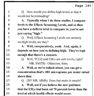
I find it intellectually dishonest to discuss something - especially teach it or use it as the basis of a report to the general public - without attempting to understand it fully.  I had no idea what an ESL or AMCV was before I read Alisa Rich's reports to the Town of Dish, Texas.  I have the same degree as Alisa Rich so we should have come up with the same understanding.  Dr. Sattler is a Ph.D dealing with ESLs.  She should understand them fully, or at the very least be able to see how it is illogical to even contemplate a health concern if the value was ".001 micrograms per metered cubed above that."

So lets look at how these two look at the ESL and the AMCV:

Q. What is your understanding of an Effects Screening Level [ESL]?

A. They are used for comparison of dispersion modeling concentrations to assess whether there could be a potential short-term or long-term health impact.

Q. And the [ESL] are used for permitting purposes; are they not?

A. That's correct.

Q, [T]hey are not ambient air concentration levels, or shouldn't be used to compare ambient air concentration levels should they?

A. They have been used that way in the past, until recently when TCEQ came out with the [AMCV], [b]ut they have come out with a new set of values that they say are appropriate to compare ambient measurements with, but the {ESL] are still the appropriate values for comparing dispersion modeling results with.

It was at this point that I started to realize that Dr. Satller did not understand the difference between using a dispersion model to predict health impacts to a receptor and using an ambient air sample to conclude possible health impacts.  What was happening here is comparing apples to oranges.  Even though an ESL looks at health impact to a receptor, when Alisa Rich placed the canister to collect the sample, she was collecting an ambient air sample.

ESLs have never been appropriate for looking at potential health impacts for an ambient air sample since they are designed for permitting purposes.  They are purposely made to be 70% more protective than what is actually required.  This is why the the TCEQ brought forward the Air Monitoring Comparison Value.  Dr. Satller was aware of this, but possibly did not understand what the 70% decrease actually means.

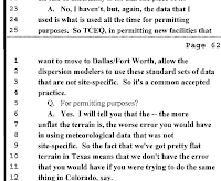
A. The TCEQ Guidance says that the [ESL] are appropriate values to use for dispersion modeling because when your doing dispersion modeling, typically you're looking at the impacts of one source.  And so the [ESL] are set lower in some cases than the [AMCV] to allow for, like, future additional sources that might move into the area that arn't accounted for in the dispersion modeling.

So you don't want one source taking up all of the air quality, [a]ll of the room in the atmosphere for emissions of that compound, because there may be future sources that move into the area that may also emit the compound.  So in some cases the ESLs are set lower than the [AMCVs].

Dr. Sattler sees it, articulates it, but does not understand it.  If the ESLs are set lower to accommodate growth, then exceeding them would not indicate a health concern, since they are designed to allow another facility into the area that would emit up to a similar amount. 

Simply put; if source A puts 2 ppb into the air, and a new source, B, puts 2 ppb into the air, than the total ppb in the ambient air would be 4 ppb.  If the ESL is 2, then it is OK for both A & B to put that amount into the air.  So if this is OK, then how should one look at the 4 ppb actually now in the air?  That's why they developed the AMCV, because the ESL is appropriate for only one source in an area and is used only for air permitting - to see what additional air pollution devices or setback may be necessary for that one source.  The dispersion modeling looks to make sure that a receptor in and around that source will not be exposed to more than the ESL form that source.

If an ambient air sample - like Alisa Rich took in the Town of Dish, Texas - has levels above the ESL, it does not indicate a health concern since the ESL is 70% lower than what is considered to be a safe level.

So, when Alisa Rich and Wilma Subra reported that the ambient levels exceeded the ESL, they were incorrect.  When Dr. Sattler produced modeling results that showed receptor concentrations above the ESL, she erred not only in how the source's emission rate was calculated but in her data's ability to now allow Alisa Rich the means whereby she could allude that there was a health issue in the Town of Dish, Texas.  Her report under "Results" states:

"The basis of an ESL is health impacts..." and "According to Table 2, short-term and long-term ESLs were exceeded for all pollutants, with the exception of long-term ESLs for styrene and toluene."

Now it is my belief that Alsia Rich knew full well how Table 2 would be interpreted by the people in the Town of DISH, Texas, as well as anyone who has a concern about oil & gas production.  All her reports are written in such a way as to not make a conclusion of yes or no, but instead are cleverly worded to be truthful without being honest.  She must - as an MPH - understand how the ESL is calculated, as should Dr. Sattler.  However, Dr. Sattler's lack of a toxicological background may preclude her understanding of Hazard Quotient (HQ) and Cancer Slope factor (see  1.6.1.1 Calculation of ESLs for Nonlinear Effects)  which might account for why she has continued down this path and, unfortunately, brought her students along with her.

To know what the model is designed to do, but completely lack an understanding of what the numbers produced mean, is just....well I don't know what to make of it.  I think the idea behind Alisa Rich's dissertation is sound - that the ratio of chemicals detected in the air might be used to determine the possible source - has potential merit.  But using the model to back in data without this fingerprinting knowledge - which was done in all three studies provided to Alisa Rich - is unsound, making all this modeling work performed by Dr. Sattler nothing more than guessing.  At the very least I will accuse her of being intellectually sloppy in her premise and her understanding of what the true health impact should be identified as.

They don't hand Ph.Ds out to just anyone, so when you have that, along with the title of "engineer" and "professor" at a "major university" by your name, it is assumed that you should have a pretty good understanding of what your are saying.  It assumes that you have spent the time necessary to thoroughly research your topic, to know it inside and out.  If her topic is air dispersion modeling, then one should reasonably expect that she fully understands what the number the model calculates means.  She doesn't, and how many people has she confused because of her failure to look at anything other than the number produced?

Numbers mean something.  The air dispersion model numbers mean something.  They are used to compare against an ESL.  She knows that.  So how in the world does she not understand what an ESL is all about?

Q. [Your 6/15/10 email states] "It seems like the TCEQ should have been using AMCVs all along as a basis of comparison for monitoring data." [S]o if someone was taking ambient air tests certainly after June of 2010, the intellectually honest thing to do would be to compare that data to AMCVs, not [ESLs] correct?

A. In my opinion.  There are people who suspect the motives of the TCEQ in issuing the AMCVs at this late date; why didn't they issue AMCVs 20 years ago?

Q. [t]he intellectually honest thing to do if you're taking air data from ambient air samples would be to compare it to that, not [ESLs] which are set 70 percent lower than the level at which health effects would be anticipated; correct?

A. I don't think the issue is that simple, because, as I said, if AMCVs were the proper thing to use, why didn't TCEQ come out with them 30 years ago.  So there are people that suspect the TCEQ's motives in issuing the AMCVs.  And if you're one of those people, you can argue that it's appropriate to go ahead and continue using the ESLs as we have - as they have been used in the past 20 years or whenever it was that they first came out with the ESLs

I'm going to interject here.  The reason they had to put the AMCVs in place is because of Alisa Rich and Dr. Sattler's misuse of them.  Prior to Alisa Rich's "reports," they were used for air permitting, not for ambient air determination of a potential problem or concern.  Alisa Rich and Wilma Subra took ambient air samples and compared those values to values that are 70% lower than what is consider to be health based.  Then, to top it off, Dr. Sattler "backs in" this ambient air data into her dispersion model and calculates potential concentrations that are, once again, compared to ESLs.  This causes the people in these communities and those around oil & gas production sites to believe that they are being harmed.  Their (TCEQ) motive was to stop this abuse/misuse.

Oh, but it gets better...so unbelievably better:

Q. Are you one of the people that suspects the TCEQ's motives?

A. I don't know.  I've worked with some people at TCEQ that are technically competent, and I've worked with some people that arn't as technically competent, so I hope that the technically competent people were involved in this decision, but I don't know for sure.

Q. When you said [i]ts reasoning seems OK," have you changed your mind about that since June 15, 2010, as you sit here today?

A: If I read the document and take it at face value, the document seems okay, but there have been some other - decisions that TCEQ has made that I think have not been technically sound since that time.

Q. Do you [h]ave any reason to think that Alisa Rich questions the motives of the TCEQ?

A. Yeah

Q. And what do you base that on?

A. Because she's been reluctant to start using the AMCVs as a basis of comparison.

Q. And why is she reluctant to use the AMCVs as a basis for comparison?

A. Because we've been using [ESLs] to compare monitoring data for the last 20, 30 years, however long the ESLs have been in existence, and so I think she questions why - why they're just now coming up with them; why didn't they come up with them 20, 30 years ago.

So maybe I was wrong to assume that Alisa Rich - who holds an MPH, like me; from a reputable University, like me; with a focus on environmental health, like me - should understand why the ESL was replaced by the AMCV for ambient air monitoring.  It's all about the HQ and the Cancer Slope Factor, the BASIC principle behind assigning risk.  The TCEQ ESL document explains it all very well.

Air dispersion modeling is all about looking at risk.  To not understand the difference between the ESL and the AMCV, is to not understand the very basis of how we look at potential adverse health effects from one source and all sources combined

Q. If you were doing an ambient air study [w]ould you use the AMCVs as the comparison value as opposed to the ESLs?

A. Yes

Q. And you would do that because you believe that would be the intellectually honest thing to do; correct?

A It would be because I would take the AMCV report at face value and - hope that the people who decided to come up with the AMCV standards were the people at TCEQ that were technically competent.

And the TCEQ, environmental professionals like me, and the general public at large, would hope that someone with a Ph.D, a job as a UTA professor, and an engineer in air dispersion modeling, would be technically competent to be able to determine this on her own and not just reluctantly accept it at "face value."

AMCVs are the correct level to use when looking at ambient air concentrations.  ESLs are used to look at what level a receptor would be exposed to if the emission rate from the source is known.  ESLs are 70% less than AMCVs because they are used for permitting.  Exceeding them does not indicate a health concern.


Next Post: Air Quality in the Barnett Shale - Part 18: Dr. Sattler's Deposition - 70% means what?


.

Air Quality in the Barnett Shale - Part 16: Dr. Sattler's Deposition - Those Seven Chemicals

In the Wolf Eagle Environmental report for the Town of Dish, Texas, Alisa Rich used values produced from dispersion modeling performed by Dr. Sattler of UTA.  These values are listed in Table 2:

Dr. Sattler's dispersion modeling maximum concentrations were developed using sampling data - collected with six SUMMA canisters possitioned a distance away from the oil & gas production site - provided by Alisa Rich.  Of these seven chemicals, two (Benzene and Toulene) are part of BTEX which is a common air pollutant derved from burring fossel fuel and cigaretts.  According to the EPA:

The primary HAP associated with the oil and natural gas production and natural gas transmission and storage source categories include BTEX and n-hexane. In addition, available information indicates that 2,2,4-trimethylpentane (iso-octane), formaldehyde, acetaldehyde, naphthalene, and ethylene glycol may be present in certain process and emission streams. Carbon disulfide (CS2), carbonyl sulfide (COS), and BTEX may also be present in the tail gas streams from amine treating and sulfur recovery units.

The State of New York identifies 1,2,4-Trimethylbenzene as a "chemical constituent" of "chemical additives proposed to be used in New York for hydraulic fracturing operations at shale wells."

This leaves styrene and dimethyl disulfide without a recognized association with oil & gas production.  Since these two chemicals were detected Alisa Rich and Dr. Sattler assume they must have come from the oil & gas production site in question and build a dispersion model as if they did.  This is why you can't back in air sample contaminant levels taken some distance from the source without first understanding what the normal background level is for the chemicals in question. There is no reason why styrene or dimethyl disulfide would be coming from this site.  Since styrene is a HAP, it would have been identified as chemicals of concern for oil & gas production MACT/GACT compliance under NESHAPS.

So lets say those two chemicals are background contaminants that came from some other process unrelated to oil & gas.  That leaves five remaining.  Both carbon disulfide and carbonyl sulfide (as well as dimethyl disulfide) were identified in the final report and in the lab reports as Tentatively Identified Compound (TICs).

This creates a bit of a problem that was not addressed in the report.  Here is what the TCEQ has to say about TICs:

TICs are observed measurements in the sample for which the gas chromatograph-mass spectrometer (GC/MS) was not specifically calibrated; however, the tentative identification of a compound can be made by comparing the mass spectrum from the environmental sample to a computerized library of mass spectra. The comparison of the sample spectra and that of the library are scored for their similarity to the mass spectrum of a particular TIC and the tentative identification is made based on the most similar spectra. This is a commonly used technique; however, the absolute identity of a TIC is uncertain. Quantifying TICs is also less accurate than for target compounds because the true relative response factor is not known, since the instrument was not calibrated for the TIC. It is important to note these uncertainties when evaluating TICs.

Given the uncertainties in identification and quantification of these compounds and the method used to determine potential 1-hour maximum concentrations, it is not possible to accurately draw conclusions about the potential for adverse health effects.

I understood why, but not to the level needed to discuss it here.  So I asked my professor over at SRPH that happens to know a little bit about analysis and GC/MS.  "It's because of the response factor" he said.  I just nodded my head making a mental note to Google that when I got back to my office.  Here is what I found to be a pretty good explanation of a Response Factor:

The size of a spectral peak is proportional to the amount of the substance that reaches the detector in the GC instrument. No detector responds equally to different compounds. Results using one detector will probably differ from results obtained using another detector. Therefore, comparing analytical results to tabulated experimental data using a different detector does not provide a reliable identification of the specimen.

A “response factor” must be calculated for each substance with a particular detector. A response factor is obtained experimentally by analyzing a known quantity of the substance into the GC instrument and measuring the area of the relevant peak. The experimental conditions (temperature, pressure, carrier gas flow rate) must be identical to those used to analyze the specimen. The response factor equals the area of the spectral peak divided by the weight or volume of the substance injected. If the technician applies the proper technique, of running a standard sample before and after running the specimen, determining a response factor is not necessary.

"Basically," he said.  "Because you did not use a standard that included these TICs, the computer makes a guess as to what chemical the peaks could represent."  He then showed me how this works by letting the computer identify an unknown bunch of peaks on a spectra he had.  The computer spat out a name.  "The lab tech needs to look at the peaks and compare it to the peaks of the compound the computer picked out.  If it's a match, great, but a lot of the time, like this example, the computer gets it wrong."

So basically what he showed me was the analytical equivalent of Damn you Auto Correct.   But they quantified these chemicals I said.  He just stared at me and then shook imaginary dice in his hands and let them fall.  I got the message.  Even if you spent the time comparing the peaks to the chemicals in the library, the lack of a standard means the quantity reported is nothing more than a guess.  Which is why the TCEQ says:

Given the uncertainties in identification and quantification of these compounds and the method used to determine potential 1-hour maximum concentrations, it is not possible to accurately draw conclusions about the potential for adverse health effects.

Well I called the lab and asked them if they physically compared the peaks found to the chemical in the library that the computer picked up.  They said no.  Damn you auto correct!

Now, to be scientific about this - which Alisa Rich should be and Dr. Sattler must be - with this information, we really need to exclude styrene, dimethyl disulfide, carbon disulfide, and carbonyl sulfide from the model.

That leaves only Benzene, Toluene, and 1,2,4-Trimethylbenzene with any reasonable plausibility for being emitted from the oil & gas production site.  Lets look at this from both a comparison to the ESL and AMCV.

Note: Toluene AMCV is for health.  ug/m3 were converted to ppbv using the formula 24.45 x concentration (ug/m3) ÷ molecular weight.  

When compared to the AMCV - which is proper in this case, and any case where air pollution permitting is not the goal -only Benzene and 1,2,4 Trimethylbenzene exceed the Annual AMCV based on the premise that these two chemicals came solely from one source only - the oil & gas production site.

So looking at it under these conditions - straightforward, fair, scientific based - what is the conclusion for the air in the Town of Dish, Texas even if these values were backed in the model?  Remember, those values reported in Table 2 are worst case possibilities.


Next Post: Air Quality in the Barnett Shale - Part 17: Dr. Sattler's Deposition - TCEQ Competency


.

Air Quality in the Barnett Shale - Part 15: Dr. Sattler's Deposition - Critique of the Method

In my last post, I discussed a Deposition I received via email regarding Dr. Melanie Sattler's involvement with Alisa Rich of Wolf Eagle Environmental (Cause No. 236-236781-09, December 14, 2010).

I find myself in another sorry-but-I-gotta-call-you-out-on-this-one position.  You see Dr. Sattler is a professor over at UTA.  She's an Engineer.  She also taught and helped Alisa Rich - who then used this association and credentials - to prepare a number of reports that are misleading (see previous posts on this topic).

In the Deposition, Dr. Sattler states:

"I think my work stands up to anybody that has expertise in dispersion modeling. If anybody was criticizing it, they probably didn't have -- well, it wouldn't surprise me to see somebody without a scientific background criticize it, because they probably wouldn't understand it." (Page 158-159)

The use of dispersion modeling to determine an emission rate is fundamentally and categorically an incorrect use of the model - unless - the contaminants being "backed in" to the equation are solely from the source - or - background levels of the contaminants have been factored out.

Here is how Dr. Satller determined the emission rate for the oil & gas production site in the Town of Dish, Texas, that Alisa Rich used to model the potential one-hour and annual exposure for those living in and around that production location:

So Alisa Rich set up seven SUMMA canisters in and around the Oil & Gas production site.  This map is included in the ZIP file titled "Revised Air Study Documents" found here.

From this graphic you might not notice all the potential sources that could be contributing to the seven contaminants reported by Alisa Rich - and supported by Dr. Sattler's work - allowing for the following statement to be made:

See those numbers in columns 2 and 5?  Those are the maximum averaged concentrations the dispersion model calculated could come from the oil & gas production site there in Dish, Texas.  Those values reported in Table 2 are what a human or environmental receptor some distance from the production site could - according to Dr. Sattles' calculations - potentially be exposed to.

So when Dr. Sattler makes that statement:

She is eluding to the fact that her modeled concentrations are so high that any error inherent in the model's ability to calculate levels of contaminants in and around the source would have no bearing on the model's conclusion that ESLs were exceeded.

This argument would be valid if you knew the actual emission rate of the source and the results obtained were high enough to overcome the percent error inherent in the model.  But in the case of Dish, Texas, her maximum contaminant levels are dependent on calculating an emission rate based on levels found in SUMMA canisters placed in and around the area where the source is located.


Because her basic premise is wrong - that you can back in the contaminant levels that were detected some distance from the source to determine the actual emission rate of the source - all the values presented in Table 2 that come from the model are wrong as well.  There is nothing wrong with the model, it's how she is using it that is wrong.  Why she can't see this, or any of her peers have not questioned her on this, is any one's guess.

There seems to be a clear lack of understanding of just what a dispersion model is capable of telling you.  Yes, she knows how they work and she knows how to report them, but she seems to lack a connection to the number obtained and how it was calculated.  Which is probably why she responded in the Deposition:

Q. When you read through [t]his report, doesn't it give you the impression that, boy, this is really bad, the air out here is just horrible?
A. I don't know.  I don't read it that way.  I look at the numbers. (page 147)

And if all you do is look at the numbers, then you are going to miss the connection to what the numbers must mean. So what do the numbers tell you?  Well based on the dispersion modelling, the air significantly exceeds the short-term and long-term ESL for six compounds.

So what Dr. Sattler accepts as good scientific methodology, is to take the sample results obtained at a distance from the source (the natural gas production area) to figure out what the emission rate coming from this source is.  Once she has this emission rate, the model can now be run like it normally is intended to be run, using all the meteorological data for a year.

Makes perfect sense, as long as you are willing to ignore all the other possible sources of these seven pollutants.  In other words, the assumption - or premise - must be that the levels of contaminants in the SUMMA canisters were solely from the natural gas production site and from no where else. 

For example, by shoving every single bit of Benzene and Toluene detected in the seven canisters back into the model's equation, an emission rate from that source was derived for Benzene and Toluene.  With that emission rate and a years worth of meteorological data, dispersion models could be run and maximum modeled concentrations (see Table 2) derived.

For these two chemicals - Benzene and Toluene - they are everywhere.  They are part of BTEX which is part of fuel, which when burned, enters the atmosphere.  Benzene also comes from smoking cigarettes.  So is it possible that not every bit of Benzene and Toluene detected in the SUMMA canisters was produced by that particular oil & gas production site?  Lets look at a map of the area:

The white rectangle is where the production site is located.  Now go back to the map showing where the sample points were located.  Isn't it possible that these contaminants could have come from other sources?

Dr. Sattler is aware of this as a potential problem:

But the Dish, Texas samples were not collected in the middle of an open field.  They were sampling air from an area where commercial activity took place, people lived, and a major thoroughfare and roads were also nearby.  Isn't it reasonable that some of that Benzene and Toluene may have come from vehicles driving on the nearby streets and FM156?  Or is that just too small of a probability to be considered?

Now if her premise is correct - that outside contaminant sources of contamination can be ignored - would this methodology - the placing of seven SUMMA canisters - work in downtown Houston?  Could you take the analytical results collected over a 24-hour period and back in to the model to derive the emission rate for one of the nearby refineries?  If not, then why is this modeling method acceptable for the Town of Dish, Texas?  You cannot reasonably make the argument for Dish that there is some small probability that maybe a little bit of the compounds came from another source.

To say that all of those seven contaminants came from one source does not even pass a grammar school understanding of how experimentation is supposed to account for bias, noise, and background.  Then, to use that emission rate to build your model whereby you can make bold sweeping statements that ESLs are exceeded by factors of, say, a thousand, is inexcusable.  You see, if the premise is wrong, then the numbers obtained are wrong - or at the very least, inconclusive.  

All models produce numbers.  All models produce numbers that - all things considered - are within a statistically acceptable level of possibility.  But not all the possible numbers produced by a model are plausible.  Intellectual integrity and the scientific method demands one know the difference. 

The numbers produced by Dr. Sattler's model are correct in terms of a calculation.  The premise, however, is wrong, making those dispersion model numbers worthless in looking at short term and long term health effects from this specific natural gas production area.


Next Post: Air Quality in the Barnett Shale - Part 16: Dr. Sattler's Deposition - Those Seven Chemicals


.