Storm Water and Texas Oil and Gas Production Facilities

A question came up from a student who had recently sat through my Storm Water Management class.

Are oil & gas facilities with SIC 1389 covered?  That SIC is identified under Section V in Sector I of the MSGP (TXR050000) as "Oil and Gas Field Services" but it indicates it is only applicable if the site had a Reportable Quantity (RQ) release since 1987? (see page 68 of the MSGP)

Interesting.....Here is what I found out.

According to the EPA:

Operators of oil and gas exploration, production, processing, or treatment operations or transmission facilities, that [were] not required to submit a permit [but had] a discharge of a reportable quantity of oil or a hazardous substance (in a storm water discharge) for which notification [to the NRC was] must apply for a [storm water] permit.

 Somehow it is the RQ that triggers EPA jurisdiction over Oil & Gas operations, but not just an RQ, an RQ "in storm water".

So are oil and gas facilities with SIC 1389 covered under the MSGP?  It depends.  Here is what the TCEQ states in the permit:

General permit coverage for oil and gas field service companies is limited to the industrial activities that occur at the service company headquarters, permanent offices, or similar base of operations.

Which means only SIC 1389 field operations do not have to apply for permit coverage.  So does this mean that oil & gas field service operations can ignore storm water and pollute it as they see fit?

No.  Instead of the MSGP, these operations must obtain an NPDES permit from the EPA if they discharge industrial storm water and be authorized by the Texas Rail Road Commission (RRC) if applicable.

Why the RRC?  According to a memorandum of understanding between the TCEQ and the RRC, it has a lot to do not just with turf, but also with the field operations themselves.

Where required by federal law, discharges of storm water associated with facilities and activities under the RRC's jurisdiction must be authorized by the EPA and the RRC, as applicable. Under 33 U.S.C. §1342(l)(2) and §1362(24), EPA cannot require a permit for discharges of storm water from "field activities or operations associated with {oil and gas} exploration, production, processing, or treatment operations, or transmission facilities" unless the discharge is contaminated by contact with any overburden, raw material, intermediate product, finished product, byproduct, or waste product located on the site of the facility.

The RRC prohibits operators from causing or allowing pollution of surface or subsurface water. Operators are encouraged to implement and maintain Best Management Practices (BMPs) to minimize discharges of pollutants, including sediment, in storm water to help ensure protection of surface water quality during storm events.

What this says is this.  Because the operator is prohibited from causing pollution to the waters of the State, a permit to discharge is not required since the water being discharged has not become contaminated by the industrial operation.  If it has, it is industrial storm water and requires an NPDES permit from the EPA.  This makes sense, since the MSGP is a permit to discharge based on the assumption that the storm water has been impacted by the industrial operation and marginally cleaned using BMPs.

OK, thats industrial, what about construction activities?

Similar logic here as well.  The memo states:

Activities under RRC jurisdiction include construction of a facility that, when completed, would be associated with the exploration, development, or production of oil or gas or geothermal resources, such as a well site; treatment or storage facility; underground hydrocarbon or natural gas storage facility; reclamation plant; gas processing facility; compressor station; terminal facility where crude oil is stored prior to refining and at which refined products are stored solely for use at the facility; a carbon dioxide geologic storage facility under the jurisdiction of the RRC; and a gathering, transmission, or distribution pipeline that will transport crude oil or natural gas, including natural gas liquids, prior to refining of such oil or the use of the natural gas in any manufacturing process or as a residential or industrial fuel.  The RRC also has jurisdiction over storm water from land disturbance associated with a site survey that is conducted prior to construction of a facility that would be regulated by the RRC.

Under 33 U.S.C. §1342(l)(2) and §1362(24), EPA cannot require a permit for discharges of storm water from "field activities or operations associated with {oil and gas} exploration, production, processing, or treatment operations, or transmission facilities, including activities necessary to prepare a site for drilling and for the movement and placement of drilling equipment, whether or not such field activities or operations may be considered to be "construction activities" unless the discharge is contaminated by contact with any overburden, raw material, intermediate product, finished product, byproduct, or waste product located on the site of the facility.  The RRC prohibits operators from causing or allowing pollution of surface or subsurface water. 

Now this has not gone on unchallenged.  In the RRC's 2009 Self-Evaluation Report they write:

In 2008 the U.S. Department of Justice filed a petition seeking rehearing of the decision by the Ninth Circuit Court of Appeals in Natural Resource Defense Council v. US E.P.A., 526 F.3d 591 (9th Cir. 2008) which vacated the U.S. EPA’s 2006 oil and gas construction storm water regulation. 

In its petition, the Government contends that the Court erred by overturning EPA’s final rule solely because the Court found it inconsistent with EPA’s prior interpretation of a provision of the Clean Water Act. The regulation effectively exempted from Clean Water Act permit requirements storm water discharges of sediment from construction activities associated with oil and gas exploration, production, processing, or treatment operations or transmission facilities unless the relevant facility had a discharge of storm water resulting in a discharge of a reportable quantity of oil or hazardous substances.

This action also encouraged voluntary application of best management practices for construction activities associated with oil and gas field activities and operations to minimize erosion and control sediment to protect surface water quality. It is unknown at this time what affect, if any, a new decision may have on RRC regulated industries.

Another one to add to "wait n' see."

Air Quality in the Barnett Shale - Part 22: Gaussian for one, Gaussian for all

I was driving home from San Antonio so I had a lot of "me" time in the car.  Instead of thinking about non-work related stuff, my brain got busy thinking about the air dispersion model used for the Town of Dish, Texas, and for the "Fort Worth League of Neighborhoods" in their report to the Fort Worth Independent School District.

All of the modeling - modeling based on the science and math behind a Gaussian dispersion - is predicated on assumptions.  Not that there is anything wrong with that, it's just that if the assumption holds true in one part it must also hold true for the rest.

So my mind is mulling this over and over.  The math behind it is daunting, especially for a guy like me, but the premise, now that is something I think I do understand.

So in the Gaussian model, which is what Dr. Sattler uses, the premise is this:

If you know the wind direction, wind speed, stack height, atmospheric conditions, and emission rate, you can estimate the plume shape and concentration of the contaminant exiting the stack at any point within the plume.

It assumes that under fixed conditions for that run - fixed air speed, fixed emission rate, fixed atmospheric conditions, fixed exhaust stack height - the plume will behave in a Gaussian manner, that is, along a fixed center line (wind direction) the plume will behave the same on each side of that line.  What these models are used for is to say, that under the most ideal conditions it would be possible for a receptor so many meters away to be potentially exposed to this much of the contaminant at that stack height and that emission rate.

Since there is nothing we can do about the wind and weather, we can adjust the stack height or adjust the emission rate to decrease the intensity of the plume for that receptor.  The emission rate is often tweaked by adding pollution control devices on the stack or limiting the production the entity can produce.  No business likes to do less production so its mostly pollution control devices that are used - or sometimes - raising the height of the stack.

In order for Dr. Sattler to generate her models, she had to assume a fixed condition as well to plug into the computer model, a model that she says uses the Gaussian formula:

She had wind and atmospheric conditions for the day of sampling, so those could be plugged in.  She could reasonably estimate the stack hight for the compressors.  What she didn't have was the actual emission rate.  So it was her reasoning, that if she had the concentration from some point in the plume, she could back in that data and calculate the emission rate that must have been in place to generate that particular concentration under these known conditions (wind speed, direction, atmospheric, stack height, plume location "y").

Now this is completely reasonable in approach.  However it is only reasonable if you assume Gaussian dispersion was taking place.  The model is for Gaussian dispersion, so to calculate an emission rate "E", Gaussian dispersion must be in place for the sample "C" used to back in to the formula.

Again, there is nothing wrong with this premise, as long as a Gaussian dispersion was in operation when the sample was collected.  In order to back in the concentration "C" to get the emission rate "E", Dr. Sattler had to have assumed Gaussian dispersion was in place, since she used a Gaussian formula to calculate the emission rate "E."

So if Gaussian dispersion was in place, and a Gaussian formula was used to calculate the emission rate "E", then the other premise of the Gaussian model is also in place as well:

That at a given emission rate "E" and a wind speed "U", and atmospheric conditions "S" and a stack height "H", somewhere on either side of that center line at location "y" you will find the contaminant to be at concentration "C."

That's when it hit me.

Nothing else is in play here in these Gaussian models.  The chemical's properties, the impact of other agents, pooling, condensing, degradation, vortexes.. they do not exist for purposes of generating these plume models.  It looks at ideal conditions to generate the modeled plume.  The model predicts maximum distance where a particular concentration of the chemical might reasonably be found.

So to "back in" the actual concentration found in a canister, the assumption must be that nothing but a Gaussian plume was being produced when the contaminant was sampled.

If that were the case, the amount of contaminants found in each canisters would be proportional, since the emission rate was steady as was everything else.  Each canister was exposed to the same wind speed "U", the same wind direction "Center Line", the same atmospheric conditions "S", and the same stack height "H".  So taking the location of the canister "y" and the concentration of the contaminant "C" and backing it in to the formula would give you "E".  That's what Dr. Sattler did because that's what she said she did in her deposition.

And with that calculated emission rate "E" she was then able to model the air for 8760 individual plumes - the number of hours in a year for which she had historical data for "U" and "S."  With that data, the emission rate "E", and the estimated stack height "H" - she was able to plug all of that into the model, and using the Gaussian plume formula, calculate both the maximum distance where the dispersion model's plume would show a concentration above a threshold (she used the ESL) as well as calculate the highest possible concentration the source could theoretically produce to which a receptor (citizen in the Town of Dish) might be exposed to.

And that's just what she did for the report, producing Table 2:

Brilliant!  Except for one little bit of a problem.  If the calculated emission rate "E" was determined by backing in the concentration "C" in to the formula, it would produce a theoretical concentration (which she averaged in columns 2 and 5).  If that holds true, then that same emission rate "E" would also be able to produce the actual concentrations in canisters 1 - 6 shown in Table 1.

If it can produce a theoretical, it should also be able to reproduce the actual - since the emission rate "E" was derived from that particular actual data.

This means that canister with the highest amount of benzene - canister 4 - must have been located in the Gaussian plume at a location "y" where the benzene would theoretically be the highest (closer to the center line) when compared to all the other canisters.  Because canister 4 has the highest benzene - because of location "y" - the model holds that at a constant emission rate "E" for the other contaminants was in play as well.

For canister 4 to produce the highest benzene concentration its location in the plume would also produce the highest concentrations for all the other contaminants. Regardless of what "E" is calculated for each contaminant, that "E" was in effect for each canister at exactly the same rate for the six contaminants being discharged on that sample day.  If any of the parameters fluctuated at any time, that impact was felt by all.  The same with wind speed, wind direction, and atmospheric conditions.  The same with stack height.  Each canister was placed and collected under the exact same conditions.  Each canister had to be in the same plume when Dr. Sattler backed in data to generate that emission rate "E."  The conditions producing the actual amount of contaminants in the six canisters must be the same if Gaussian dispersion was in play.

Unless it wasn't.

And if you look at Table 2, you will clearly see it was not.  So if Gaussian dispersion was not taking place that day, then how can you back in the data to calculate an emission rate from a formula that is based on showing a Gaussian dispersion?  If the emission rate "E" that Dr. Sattler calculated cannot be used to calculate the actual concentrations seen, then how can it be used to calculate a theoretical maximum?

And if you ignore that by explaining it away saying the actual concentrations in the six canisters were impacted by other conditions, then you are admitting that Gaussian dispersion was not in play, therefore an emission rate "E" cannot be calculated since no other variables are considered in the formula.

And if you say the sample was collected over 24 hours and was diluted, well that doesn't affect Gaussian dispersion since all the samples were collected for that same period and would have been similarly diluted.

And if you say the wind conditions changed for each of the canisters throughout the day impacting the concentrations of some of the contaminants getting to the canisters, well then, you are really grasping at straws.  And besides, if that's the case, how do you know what concentration to back in to the model?

There are two equally valid reasons why Dr. Sattler's modeling and the subsequent "averaged concentrations" are incorrect:

1. It is impossible to calculate the exact concentration attached to a particular "y" to back into the model because - in real life - the plume is consistently changing over time.  Gaussian modeling assumes perfect and steady conditions in order to produce a plume.  So "E" can never accurately be calculated by backing in the concentration.
2. The concentrations captured in the six canisters came from multiple sources and not from one source as modeled.  In this case, backing those concentrations into the model will always generate an emission rate "E" that is higher than what it is.  This incorrect "E" will then generate plumes and concentrations that are also too high.

Bottom line is this:

If you assume Gaussian dispersion modeling can reasonably model possible concentrations within a plume....

....and you assume that the formula for ground level concentrations is correct:

....and you agree that the canisters were all under the same wind speed, wind direction, and atmospheric conditions...

....and the emission rate "E" was exactly the same for each of the contaminants detected in each of the six canisters...

....and you accept that the emission rate, along with all the other parameters, plugged into that formula will produce a plume that is Gaussian (see graphic at the beginning)....

....then the plume produced from that calculated emission rate "E" must accurately match the actual concentrations found in the six canisters in and around that modeled plume....

...and if the modeled plume - using to emission rate obtained by backing in the actual concentration - does not reproduce the actual concentration that were used to derive it....

....then either the model is wrong....

...or the samples have been impacted by conditions not considered in a Gaussian model....

...which means that the actual concentration found in the six canisters cannot be used to calculate the emission rate of the source....

....which means the data presented in Table 2 of the report, as well as any other report produced using backed in data to find an emission rate, is incorrect.

Bottom-bottom line.

As it stands now, Dr. Sattler's methodology of "backed in" data cannot be used to calculate an emission rate in order to generate plume data to show modeled average concentration levels and/or determine the proper setback for a source.

Bottom-bottom-bottom line:

You cannot use non-Gaussian data to determine the value needed in a formula that produces a Gaussian model.


Next post: The Fort Worth League of Neighborhoods Report to FWISD - Different place, same drummer


.

Air Quality in the Barnett Shale - Part 21: If you assume E to be...

So in my last post I attempted to explain how the Gaussian model works based on my limited knowledge of the math - or math in general for that matter!

I am pretty sure that to "back in" to the model, the concentration "C" to obtain the emission rate "E," you have to know the values for all the other parameters in the formula:

So Dr. Sattler knows "C", she knows the distance from the stack where the sample was collected - "x".  She has the wind speed "U" and the meteorological data for the two S parameters.  She can estimate the height of the stack "H" and she knows, pi.  The only variable she does not know is "y" which needs to be calculated from the center line - required if the Gaussian principle is to be true - and the distance from the source "x."

The only way to get "y" is to fix the center line in one direction - which would be the wind direction - in order for the Gaussian model to hold true and a dispersion plume to be generated:

At a fixed wind direction, the stack at time = 0 will have the x,y coordinates of 0,0.  "y" is some distance from the stack - one side or the other (does not matter in a Gaussian model - both sides assumed equal in concentration) on the y-coordinate of the graph.

So in the Town of Dish example, here is what we are looking at.  Lets assume the wind is blowing in a Northwest direction.  That would be the center line.

Now I am going to orientate the map so it is in the same direction as the "Top View" plume graphic above:

If we know where the center line from the source is to be placed (wind direction), we can get the x,y coordinates.  With that data, the emission rate "E" can be calculated according to Dr. Sattler.

But that creates a problem....If we assume the Gaussian model to be true, and we assume the "backed in" data can calculate an emission rate "E", and the Gaussian model predicts a concentration at an x,y coordinate based on a wind speed "U" of meters per second and an emission rate "E" of grams per second, then logic would hold that the highest level of benzene would also show the highest levels of the other constituents in that sample point.

Look at Table 1:

In order to claim all of the contaminants in the six canisters came from one source at x,y = 0,0...then the model would predict similar ratios in every sample.  If you were to argue that the wind direction changed - thereby changing the center line - the same principle would hold true under the Gaussian model, that is, if you had low benzene you would also have low carbon disulfide, or if you had high carbon disulfide and low benzene in one sample you would have a similar ratio in the rest.  That's if you consider the Gaussian model to be true.

So either the Gaussian model is wrong in its "heart of the calculation" or the samples contain concentrations of chemicals from more than one source - which - if that the case, the emission rate "E" that was calculated is way too high thereby making all the dispersion model maps and concentrations calculated from it too high as well.

Or maybe wind direction moves all over the place changing the concentrations in the x,y coordinates where the samples were collected over a 24 hour period making it impossible to accurately "back in" to the model to get an emission rate since you would never know where the center line was.

I wonder which one it could be...

As ignorant as I most likely am on dispersion modeling, Dr. Sattler's premise and her emission calculations and dispersion modeling based on that value is wrong.  And that's not even bringing into the overall equation the use of TICs and the fact that all of this is based on a one time sampling event (n=1).

Somethin' aint right about all this.


Next Post: Air Quality in the Barnett Shale - Part 22: Gaussian for one, Gaussian for all.
.

Air Quality in the Barnett Shale - Part 20: Dr. Sattler's Deposition - The Gaussian Model

Well I thought I was done with this topic...but something occurred to me when I was reviewing a presentation on air dispersion modeling a friend of mine gave me.  Let me be clear on this up front.  I don't know nothin' about air dispersion modeling.  Math makes my head hurt.  However, I can sometimes look at something complex and get some semblance of understanding.

So Dr. Sattler in her Deposition stated that the air dispersion program was based on a Gaussian dispersion model:

What that means, is that the plume of chemicals (the smoke so-to-speak) coming from the end of the pipe (the smoke stack) behaves in a Gaussian manner:

In other words, if the wind direction stays constant, and the emission rates stays constant, and all the other atmospheric conditions stay constant, we can estimate the concentration at some point away from the stack:

This is based on the formula - what Dr. Sattler states is the "heart of the computer software" - which looks like this:

Because the samples were taken at "ground level" we use the formula to calculate a "ground level" concentration:

Does your head hurt yet?  Mine does....but bear with me.

So, for example under "normal" atmospheric conditions, this particular plume - over time - would look like this:

...and under "unstable" conditions we would expect it to look like this"

What this shows is...that with a smoke stack that is 25 meters high, a wind speed of 1 meter per second, and an emission rate coming out of the smoke stack of 1 gram of chemical per second, we would expect some concentration near what is modeled at some distance away from the stack in the "x" direction and some distance away in the "y" direction.  The wind direction stays constant - that's the center line - and x and y are some point around that center line line.

So if I know the stack hight, the wind speed, and the emission rate, and I know the atmospheric conditions, the concentration "C" at x and y distance at 0 - or ground "z" - can be estimated.

That's what Dr. Sattler did for Alisa Rich, only she did with 8760 hours of meteorological data provided to her:

But first she needed to calculate the emission rate "E."  And that's when it hit me...

To "back in" the concentration C(x,y,z) to get E, certain parameters needed to be fixed.  Dr. Sattler could estimate the stack hight "H," and she knew the canister was collected at ground level, so z = 0.  She also had the atmospheric conditions and wind speed for the 24 hours of the time the sample was collected.

And here is where I started to see a problem.  She has a sample that is fixed - it stayed in one spot and collected a sample over 24 hours.  The dispersion model tells you what the concentration will be at some distance away from the stack, that is, if I grab a sample at an x-y coordinate, I would would expect a concentration of C.  But the samples in which the the data on concentration was obtained to "back in" was many grab samples all collected and added together.

What's the problem with that?  Well in order for the Gaussian model to work, it assumes a center line:

So at an emission rate "E" of, lets say, 1 gram per second, and a wind speed "U" of 1 meter per second, at 10 meters in the direction of that center line, 10 grams have been released, with the concentration highest at the stack.  Now as the atmospheric conditions change - stable - unstable - how far that plume is dispersed will vary (see the two example above).

What this means...is in order for Dr. Sattler to "back in the concentration, she had to fix the wind direction (the center line).  So based on the wind direction chosen, the variable "y" can be determined.  But what concentration do you use for that x-y position?  Because the x-y concentration at a fixed z = 0, is a matter of wind speed and emission rate.  Since we know the wind speed, did she assume the total concentration collected over 24 hours was what determined that emission rate?

In other words, to get the benzene concentration of canister 4 (Table 1) that was located x and y distance from the source, with a known wind speed of "U", the emission rate "E" would be artificially high if it was backed in, since in the model, at x-y distance at wind speed "U" and emission rate "E", the concentration "C" is predicted to be at some value.  

Since we know that value "C" and we know the wind speed "U", and we know the x-y coordinates of the sample canister, I am wondering if she set "E" based on the 24 hour concentration?  If that's how she did it, then "E" in all other model days would be extremely inflated.  It is possible that she compensated for this by knowing how much time elapsed based on the wind speed to get from the source to the canister - and then divided the 24 hour concentration by that time frame to get an average.

But even if that was done, there is another problem with her premise of "backed in" data and the Gaussian model's assumptions...

My head really hurts now....

Next post: Air Quality in the Barnett Shale - Part 21: Dr. Sattler's Deposition - If you assume E to be...

.

Air Quality in the Barnett Shale - Part 19: Dr. Sattler's Deposition - Down with bad science!

Here is why I am critical of the work performed by Alisa Rich of Wolf Eagle Environmental and Dr. Sattler, of UTA.

From Fort Worth's NBC station:

"When you start actually looking at the levels of carbon disulfide, it's shocking," said Deborah Rogers, who has been involved in the league and monitoring natural gas drilling for the last several years. "People are going to be concerned."

Please read my post on TICs.  It is doubtful that carbon disulfide is present in the air.  Carbon disulfide is a TIC and is not positively identified nor is it quantified in the GC/MS test method used for the other contaminates.

The study makes the following recommendations for all Fort Worth ISD leases going forward:

1.Setbacks of approximately one mile from the school boundaries are needed to ensure that emissions of carbon disulfide (neurotoxin), benzene (carcinogen) and other drilling toxics do not exceed 8 hour limits for short term health benchmarks (See Dispersion Modeling Results).

Now whether setbacks are appropriate is not being questioned by me.  However, basing the one-mile setback on work performed by Rich and Sattler is.  Carbon disulfide is a TIC and its identity and quantification unverifiable.  Benzene concentrations from ambient air samples were backed in to the air dispersion model - generating an emission rate for that source.  Background benzene - that which is not from the source being modeled - was also included in this calculation generating a potential emission rate that would be higher than if the actual emission rate was known.  See my post on backed in data

Furthermore, Rich and Sattler compared these model contaminant levels to ESLs -which are for permitting and 70% lower than they need to be - and not to AMCVs - which are for ambient air.  See my post on ESLs & AMCVs.

Now I am in favor of a lot of the proposed requirements, such as green completions and substitution for toxic chemicals (depending on cost/benefit).  I think they are within reason, and if everyone is required to do them, that cost can be factored in as the cost of doing business.

So here is what really bothers me about bad science and those that should know better willingly feeding it as fact to the masses.

From the Star-Telegram Barnett Shale Blog

DISH Mayor Calvin Tillman, an outspoken critic of current drilling practices in the Barnett Shale, was the subject of a story in the Philadelphia Inquirer last week.  The story ends with a peek into Tillman's latest worry: 

Though Tillman's blood and urine came in below levels expected for the general population, he is still worried. "I'm not sure I'm going to be able to live here," he said earlier this week.

Tillman's water tested positive for traces of three contaminants, all below federal legal limits for public water: styrene was 3,700 times below the limit; ethylbenzene was 28,000 times below the limit, and xylenes were 47,393 times below the legal limit.

"The most disturbing is the toxins found in our water," Tillman said in an e-mail. "They should not be there at all. Not sure what to do about that."

Well I can tell you what you should not do about that.  Don't contact Alisa Rich, Wilma Subra, Dr. Sattler, or Wolf Eagle Environmental for advice.

You see, even when there is nothing there some people still worry.  So giving others this worry by telling them something is there does nothing more than bring in consulting dollars while causing more worry.

And from a public health point of view, worry causes stress, stress causes disease.  The worry over nothing is more likely to harm you than the air or water you are exposed to at your home.

Here's to good science in the future.


Next Post: Air Quality in the Barnett Shale - Part 20: Dr. Sattler's Deposition - The Gaussian Model

.

Air Quality in the Barnett Shale - Part 18: Dr. Sattler's Deposition - 70% means what?

For the last four posts I've been looking at how Alisa Rich with Wolf Eagle Environmental and Dr. Sattler with UTA could have concluded that the results of air dispersion modeling performed on six ambient air samples collected over a 24-hour period indicated a problem with the air the good people of the Town of Dish, Texas, were having to breath now that a bunch of gas compressors were located in their town.

I've been critical of their work on many fronts, but it all seems to revolve around the use of ESLs to compare ambient air samples.  This is not what ESLs are to be used for, but Alisa Rich, with the assistance of Dr. Sattler, decided that it would be appropriate to use them in their reports.

The two of them have been unable to get their heads wrapped around why the ESL shouldn't be used, going so far as to accuse the TCEQ of not being technically competent when they tried to rectify this misuse with the issuance of the AMCV for ambient air samples, like the ones collected by Alisa Rich.

In their thinking, a value that is 70% lower than another must be, somehow, more safe.

So is the ESL that is 70% lower than this new AMCV value the TCEQ wants to use a better value to use?

No.


ESLs and AMCVs are based on an inhalation Reference Value (ReV) which is defined:

[a]s an estimate of an inhalation exposure concentration for a given duration to the human population (including susceptible subgroups) that is likely to be without an appreciable risk of adverse effects. ReVs are based on the most sensitive adverse health effect relevant for humans reported in the literature.

For non-cancer causing chemicals and chemicals that show a nonlinear effect, the formula:

• (acute)ESL = 0.3 x (acute)ReV
• (chronic)ESL = 0.3 x (chronic)ReV
• (acute)AMCV = (acute)ReV
• (chronic)AMCV = (chronic)ReV

For chemicals suspected to cause cancer the ESL and AMCV are the same.

The ESL is one third the ReV.  And the ReV is the value which is based on the most sensitive adverse health effects relevant for humans.

So if the AMCV = the ReV, and the ReV is the value which is based on the most sensitive adverse health effects relevant for humans, will lowering the value by 70% bring about any more protection?

No.

Another way to look at it is like this:  If the maximum temperature that a hot tub will go is 104F, is 104F the maximum temperature deemed safe for humans?

Yes.

If we lower the temperature to 90F, will we have made it any more safer?  How about to 65F?

No.

Now the thing about temperature is this.  If you add 90F water to 90F water, the water will be 90F.  But if you add 60 ppb of Benzene from one source with 60 ppb of Benzene from another source, you could get 120 ppb of Benzene in the ambient air.

If the ESL for Benzene is 54 ppb, the two sources would be putting more Benzene into the air than they should, but it would still be at a safe level.  Even when the two concentrations are added together (120 ppb) it is still safe because 120 is less than the ReV which is 180 ppb.

And you know what the AMCV for short term Benzene is?  180 ppb.

Since Benzene is also a suspected carcinogen, the long-term (chronic) level is set to 1.4 ppb for an average over a lifetime for both the ESL and the AMCV.

So there you have it.  You could be exposed to 180 ppb for up to one hour with no adverse health effects and as long as your average (for a lifetime) does not exceed 1.4 ppb, you should have no adverse health effects from Benzene.

That's how it works.

Now go check the TCEQ's ambient air monitoring web site to see what the one-hour levels for Benzene are. (make sure to check; measured in ppb-v, clear all checkboxes, check benzene, generate report)

I'll wait.

See?  Feel better now?

So just so we are clear on this.  The AMCV is the ReV.  The ReV is based on the most sensitive adverse health effect relevant for humans reported in the literature.  The ESL is 70% lower than the AMCV.

Next Post: Air Quality in the Barnett Shale - Part 19: Dr. Sattler's Deposition - Down with bad science!

.

Air Quality in the Barnett Shale - Part 16: Dr. Sattler's Deposition - Those Seven Chemicals

In the Wolf Eagle Environmental report for the Town of Dish, Texas, Alisa Rich used values produced from dispersion modeling performed by Dr. Sattler of UTA.  These values are listed in Table 2:

Dr. Sattler's dispersion modeling maximum concentrations were developed using sampling data - collected with six SUMMA canisters possitioned a distance away from the oil & gas production site - provided by Alisa Rich.  Of these seven chemicals, two (Benzene and Toulene) are part of BTEX which is a common air pollutant derved from burring fossel fuel and cigaretts.  According to the EPA:

The primary HAP associated with the oil and natural gas production and natural gas transmission and storage source categories include BTEX and n-hexane. In addition, available information indicates that 2,2,4-trimethylpentane (iso-octane), formaldehyde, acetaldehyde, naphthalene, and ethylene glycol may be present in certain process and emission streams. Carbon disulfide (CS2), carbonyl sulfide (COS), and BTEX may also be present in the tail gas streams from amine treating and sulfur recovery units.

The State of New York identifies 1,2,4-Trimethylbenzene as a "chemical constituent" of "chemical additives proposed to be used in New York for hydraulic fracturing operations at shale wells."

This leaves styrene and dimethyl disulfide without a recognized association with oil & gas production.  Since these two chemicals were detected Alisa Rich and Dr. Sattler assume they must have come from the oil & gas production site in question and build a dispersion model as if they did.  This is why you can't back in air sample contaminant levels taken some distance from the source without first understanding what the normal background level is for the chemicals in question. There is no reason why styrene or dimethyl disulfide would be coming from this site.  Since styrene is a HAP, it would have been identified as chemicals of concern for oil & gas production MACT/GACT compliance under NESHAPS.

So lets say those two chemicals are background contaminants that came from some other process unrelated to oil & gas.  That leaves five remaining.  Both carbon disulfide and carbonyl sulfide (as well as dimethyl disulfide) were identified in the final report and in the lab reports as Tentatively Identified Compound (TICs).

This creates a bit of a problem that was not addressed in the report.  Here is what the TCEQ has to say about TICs:

TICs are observed measurements in the sample for which the gas chromatograph-mass spectrometer (GC/MS) was not specifically calibrated; however, the tentative identification of a compound can be made by comparing the mass spectrum from the environmental sample to a computerized library of mass spectra. The comparison of the sample spectra and that of the library are scored for their similarity to the mass spectrum of a particular TIC and the tentative identification is made based on the most similar spectra. This is a commonly used technique; however, the absolute identity of a TIC is uncertain. Quantifying TICs is also less accurate than for target compounds because the true relative response factor is not known, since the instrument was not calibrated for the TIC. It is important to note these uncertainties when evaluating TICs.

Given the uncertainties in identification and quantification of these compounds and the method used to determine potential 1-hour maximum concentrations, it is not possible to accurately draw conclusions about the potential for adverse health effects.

I understood why, but not to the level needed to discuss it here.  So I asked my professor over at SRPH that happens to know a little bit about analysis and GC/MS.  "It's because of the response factor" he said.  I just nodded my head making a mental note to Google that when I got back to my office.  Here is what I found to be a pretty good explanation of a Response Factor:

The size of a spectral peak is proportional to the amount of the substance that reaches the detector in the GC instrument. No detector responds equally to different compounds. Results using one detector will probably differ from results obtained using another detector. Therefore, comparing analytical results to tabulated experimental data using a different detector does not provide a reliable identification of the specimen.

A “response factor” must be calculated for each substance with a particular detector. A response factor is obtained experimentally by analyzing a known quantity of the substance into the GC instrument and measuring the area of the relevant peak. The experimental conditions (temperature, pressure, carrier gas flow rate) must be identical to those used to analyze the specimen. The response factor equals the area of the spectral peak divided by the weight or volume of the substance injected. If the technician applies the proper technique, of running a standard sample before and after running the specimen, determining a response factor is not necessary.

"Basically," he said.  "Because you did not use a standard that included these TICs, the computer makes a guess as to what chemical the peaks could represent."  He then showed me how this works by letting the computer identify an unknown bunch of peaks on a spectra he had.  The computer spat out a name.  "The lab tech needs to look at the peaks and compare it to the peaks of the compound the computer picked out.  If it's a match, great, but a lot of the time, like this example, the computer gets it wrong."

So basically what he showed me was the analytical equivalent of Damn you Auto Correct.   But they quantified these chemicals I said.  He just stared at me and then shook imaginary dice in his hands and let them fall.  I got the message.  Even if you spent the time comparing the peaks to the chemicals in the library, the lack of a standard means the quantity reported is nothing more than a guess.  Which is why the TCEQ says:

Given the uncertainties in identification and quantification of these compounds and the method used to determine potential 1-hour maximum concentrations, it is not possible to accurately draw conclusions about the potential for adverse health effects.

Well I called the lab and asked them if they physically compared the peaks found to the chemical in the library that the computer picked up.  They said no.  Damn you auto correct!

Now, to be scientific about this - which Alisa Rich should be and Dr. Sattler must be - with this information, we really need to exclude styrene, dimethyl disulfide, carbon disulfide, and carbonyl sulfide from the model.

That leaves only Benzene, Toluene, and 1,2,4-Trimethylbenzene with any reasonable plausibility for being emitted from the oil & gas production site.  Lets look at this from both a comparison to the ESL and AMCV.

Note: Toluene AMCV is for health.  ug/m3 were converted to ppbv using the formula 24.45 x concentration (ug/m3) ÷ molecular weight.  

When compared to the AMCV - which is proper in this case, and any case where air pollution permitting is not the goal -only Benzene and 1,2,4 Trimethylbenzene exceed the Annual AMCV based on the premise that these two chemicals came solely from one source only - the oil & gas production site.

So looking at it under these conditions - straightforward, fair, scientific based - what is the conclusion for the air in the Town of Dish, Texas even if these values were backed in the model?  Remember, those values reported in Table 2 are worst case possibilities.


Next Post: Air Quality in the Barnett Shale - Part 17: Dr. Sattler's Deposition - TCEQ Competency


.

Air Quality in the Barnett Shale - Part 15: Dr. Sattler's Deposition - Critique of the Method

In my last post, I discussed a Deposition I received via email regarding Dr. Melanie Sattler's involvement with Alisa Rich of Wolf Eagle Environmental (Cause No. 236-236781-09, December 14, 2010).

I find myself in another sorry-but-I-gotta-call-you-out-on-this-one position.  You see Dr. Sattler is a professor over at UTA.  She's an Engineer.  She also taught and helped Alisa Rich - who then used this association and credentials - to prepare a number of reports that are misleading (see previous posts on this topic).

In the Deposition, Dr. Sattler states:

"I think my work stands up to anybody that has expertise in dispersion modeling. If anybody was criticizing it, they probably didn't have -- well, it wouldn't surprise me to see somebody without a scientific background criticize it, because they probably wouldn't understand it." (Page 158-159)

The use of dispersion modeling to determine an emission rate is fundamentally and categorically an incorrect use of the model - unless - the contaminants being "backed in" to the equation are solely from the source - or - background levels of the contaminants have been factored out.

Here is how Dr. Satller determined the emission rate for the oil & gas production site in the Town of Dish, Texas, that Alisa Rich used to model the potential one-hour and annual exposure for those living in and around that production location:

So Alisa Rich set up seven SUMMA canisters in and around the Oil & Gas production site.  This map is included in the ZIP file titled "Revised Air Study Documents" found here.

From this graphic you might not notice all the potential sources that could be contributing to the seven contaminants reported by Alisa Rich - and supported by Dr. Sattler's work - allowing for the following statement to be made:

See those numbers in columns 2 and 5?  Those are the maximum averaged concentrations the dispersion model calculated could come from the oil & gas production site there in Dish, Texas.  Those values reported in Table 2 are what a human or environmental receptor some distance from the production site could - according to Dr. Sattles' calculations - potentially be exposed to.

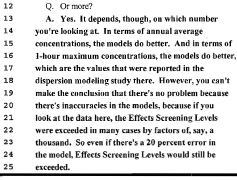
So when Dr. Sattler makes that statement:

She is eluding to the fact that her modeled concentrations are so high that any error inherent in the model's ability to calculate levels of contaminants in and around the source would have no bearing on the model's conclusion that ESLs were exceeded.

This argument would be valid if you knew the actual emission rate of the source and the results obtained were high enough to overcome the percent error inherent in the model.  But in the case of Dish, Texas, her maximum contaminant levels are dependent on calculating an emission rate based on levels found in SUMMA canisters placed in and around the area where the source is located.


Because her basic premise is wrong - that you can back in the contaminant levels that were detected some distance from the source to determine the actual emission rate of the source - all the values presented in Table 2 that come from the model are wrong as well.  There is nothing wrong with the model, it's how she is using it that is wrong.  Why she can't see this, or any of her peers have not questioned her on this, is any one's guess.

There seems to be a clear lack of understanding of just what a dispersion model is capable of telling you.  Yes, she knows how they work and she knows how to report them, but she seems to lack a connection to the number obtained and how it was calculated.  Which is probably why she responded in the Deposition:

Q. When you read through [t]his report, doesn't it give you the impression that, boy, this is really bad, the air out here is just horrible?
A. I don't know.  I don't read it that way.  I look at the numbers. (page 147)

And if all you do is look at the numbers, then you are going to miss the connection to what the numbers must mean. So what do the numbers tell you?  Well based on the dispersion modelling, the air significantly exceeds the short-term and long-term ESL for six compounds.

So what Dr. Sattler accepts as good scientific methodology, is to take the sample results obtained at a distance from the source (the natural gas production area) to figure out what the emission rate coming from this source is.  Once she has this emission rate, the model can now be run like it normally is intended to be run, using all the meteorological data for a year.

Makes perfect sense, as long as you are willing to ignore all the other possible sources of these seven pollutants.  In other words, the assumption - or premise - must be that the levels of contaminants in the SUMMA canisters were solely from the natural gas production site and from no where else. 

For example, by shoving every single bit of Benzene and Toluene detected in the seven canisters back into the model's equation, an emission rate from that source was derived for Benzene and Toluene.  With that emission rate and a years worth of meteorological data, dispersion models could be run and maximum modeled concentrations (see Table 2) derived.

For these two chemicals - Benzene and Toluene - they are everywhere.  They are part of BTEX which is part of fuel, which when burned, enters the atmosphere.  Benzene also comes from smoking cigarettes.  So is it possible that not every bit of Benzene and Toluene detected in the SUMMA canisters was produced by that particular oil & gas production site?  Lets look at a map of the area:

The white rectangle is where the production site is located.  Now go back to the map showing where the sample points were located.  Isn't it possible that these contaminants could have come from other sources?

Dr. Sattler is aware of this as a potential problem:

But the Dish, Texas samples were not collected in the middle of an open field.  They were sampling air from an area where commercial activity took place, people lived, and a major thoroughfare and roads were also nearby.  Isn't it reasonable that some of that Benzene and Toluene may have come from vehicles driving on the nearby streets and FM156?  Or is that just too small of a probability to be considered?

Now if her premise is correct - that outside contaminant sources of contamination can be ignored - would this methodology - the placing of seven SUMMA canisters - work in downtown Houston?  Could you take the analytical results collected over a 24-hour period and back in to the model to derive the emission rate for one of the nearby refineries?  If not, then why is this modeling method acceptable for the Town of Dish, Texas?  You cannot reasonably make the argument for Dish that there is some small probability that maybe a little bit of the compounds came from another source.

To say that all of those seven contaminants came from one source does not even pass a grammar school understanding of how experimentation is supposed to account for bias, noise, and background.  Then, to use that emission rate to build your model whereby you can make bold sweeping statements that ESLs are exceeded by factors of, say, a thousand, is inexcusable.  You see, if the premise is wrong, then the numbers obtained are wrong - or at the very least, inconclusive.  

All models produce numbers.  All models produce numbers that - all things considered - are within a statistically acceptable level of possibility.  But not all the possible numbers produced by a model are plausible.  Intellectual integrity and the scientific method demands one know the difference. 

The numbers produced by Dr. Sattler's model are correct in terms of a calculation.  The premise, however, is wrong, making those dispersion model numbers worthless in looking at short term and long term health effects from this specific natural gas production area.


Next Post: Air Quality in the Barnett Shale - Part 16: Dr. Sattler's Deposition - Those Seven Chemicals


.

Air Quality in the Barnett Shale - Part 11: Is there a real concern for DISH, Texas?

So what do we know so far regarding the real health concerns for the citizens of the Town of DISH, Texas?:

• Benzene and other chemicals were found in the seven samples collected during one 24 hour sampling event conducted by Wolf Eagle Environmental.
• The TCEQ has sampled the air in the Town of DISH, Texas and reports hourly values below the short-termAir Monitoring Comparison Values (AMCV)  
• The TCEQ has sampled the air in the Town of DISH, Texas and reports hourly values below the short-termAir Monitoring Comparison Values (AMCV)  

Here is what I gathered from the TCEQ website for air monitoring at DISH, Texas:

Note: Report generated on Dec 16, 2010.  Monthly and Yearly data reported for BTEX.

As you can see, the amount of BTEX (Benzene, Toluene, Ethylbenzene, and Xylene) is under the AMCV for each chemical.  That's a good sign.  But lets make the assumption that the 24 hour results reported by Wolf Eagle Environmental are what the citizens of DISH, Texas are being exposed to on a regular basis.  Would there be a health concern?

That's a difficult one to make a call on.  In fact it is so uncertain that even Wolf Eagle Environmental and Wilma Subra in any of their reports do not make any claim what-so-ever as to these levels creating a undo health risk.  All that is said is that they exceed the ESL for some of the chemicals found.

The TCEQ, on the other hand, does state:

"24-hour air monitors in the Barnett Shale area are showing no levels of concern for any chemicals." and "there are no immediate health concerns from air quality in the area" and "that when they are properly managed and maintained, oil and gas operations do not cause harmful excess air emissions.”

Now I know better than to rest my case on one set of data.  However, I have at my disposal - and anyone clicking the links I cite does as well - a whole bunch of data or 'n'.  This gives me more confidence to agree with the statement TCEQ has issued above.

There is one more issue in play that leads me to conclude that the air is safe and that the folks in the Town of DISH, Texas are not going to experience " health concerns from air quality in the area."

Exposure is but one step of the K.C.Donnelly Risk Paradigm I discussed in Part 2.

What needs to happen after exposure to a chemical takes place is uptake.  That is, the chemical has to enter into the body where the dose, time, and pharmacokinetics now come into play.

The question becomes, OK, if they are exposed, how much are they actually getting into their system?  In order for a health effect to manifest, uptake must take place.  And if uptake has taken place, we can measure the actual concentration of the chemical in the blood stream or tissue.

And wouldn't you know it, that has been done.

Much of the concern about natural gas operations has been centered in DISH, so in early 2009, the Texas Department of State Health Services performed blood tests on 28 DISH residents (representing about 13 percent of the town’s population).

Test results showed that the exposure of DISH residents to VOCs was similar to that of the general U.S. population, and that exposure to certain contaminants was no higher than that of the general U.S. population.

The study further found that the only residents who had higher levels of benzene in their blood were smokers. Cigarette smoke contains benzene, so finding this in smokers’ blood is not unusual, the department noted. (1)

So now what do we know?

• We know that we have detected chemicals contaminants in the 24 hour samples collected by Wolf Eagle Environmental
• We can assume exposure has taken place.
• We can show - through blood tests - that exposed citizens have levels of contaminants no higher than those of the general US population.

So what can we conclude from all this?  That excluding odor, noise, and catastrophic events, the TCEQ is correct in asserting "that when they are properly managed and maintained, oil and gas operations do not cause harmful excess air emissions.”


Next Post: Air Quality in the Barnett Shale - Part 12: Oil & Gas, it's better if you go green!

.

Air Quality in the Barnett Shale - Part 8: Benzene is like a bull...

So those last two posts were a bit on the scientific side.  However, if I am going to be critical on someone else's report lacking credibility and good science, I need to be ably to show why.  So with cheesy graphics, let me see if I can 'splain it a little bit better.

Let's deal with Benzene first, since it is recognized as a human carcinogen.

Lets say I lived in a house that boarders a very large pasture.  Surrounding this pasture are three other neighbors.  My neighbors and I walk along a well traveled path through the field to the town hall, where we all like to meet nightly to socialize and whittle sticks into pointy spears.

One day this well-dressed out-of-towner shows up at our town hall and offers us a bunch of money if we would lease him part of our pasture.  Liking money, we all say "yes" except neighbor three.

"I heard about him" neighbor 3 says, "He sets up on our town and lets loose bulls and rams in our pasture!  I think we need to do a little bit more research before we say yes to this offer."

"Well I just looked it up on the Google," neighbor 2 yells excitedly.  "Says on the Internet that living near bulls and rams can bring all sorts of harm.  In fact, bulls are known to gouge which can become infected causing death!  I have two small children that walk in that pasture!  I'm going to have to say 'no' now"

"Hold on a minute!" neighbor 1 says a bit perturbed.  "I've been around bulls and rams all my life, and nothing has ever happened to me!  I don't know what y'all are afraid of, look at the money we would all be getting?  So what if they add some bulls and rams to our pasture.  It's worth it in my opinion."

"I have a suggestion" I say.  "Why don't we contact one of those Bullologists from the local University and see what an expert has to say."

The next day, a man looking just like a college professor, shows up at our town hall and tells us his name is Professor Paracelsus.  "Call me Dr. P" he says with a smile.

"So the concern is over the bulls and rams that this out-of-town fellow will be adding to your pasture," Dr. P says.  "I can see you have been researching this on the Internet and have little doubt why some of you are now very afraid.  Let's look at the rams first shall we."

"We look at exposure to rams and bulls..." Dr. P continued, "...based on their acute (short-term) and chronic (long-term) adverse effects.  We then determine the number of bulls and rams a person can be exposed to - called a dose - and the health effect that will result - called the response."

"Because rams have horns that bend inward they are unable to gouge you if you come in contact with one.  No gouging means no infection.  Now rams can still cause harm, but you need a bunch of them.  One can knock you over, but the only way you can be seriously hurt is if a bunch trample over you.

"Now the number we determine will cause harm is dependent on the population that will be exposed.  Young children, older folks, and those that are sick are most vulnerable to being trampled so we set the "safe" amount of rams you can be around daily based on this.  This dose-response level is called a threshold or Reference Value (ReV) -  a dose below which no effect is observed. In scientific terms, we call this a non-linear nonlinear dose-response relationships."

"Acute ReVs are the number of non-gouging animals a person can be exposed to and are typically derived for a 1-hour exposure time with that animal.   Chronic ReVs are are derived for a lifetime exposure duration to non-gouging animals and assume that constant exposure that causes bruising, sprains and broken bone may cause arthritis or amputations in a person's later years."

"So being exposed periodically to rams will allow for a much higher number than if you were to constantly be exposed to them throughout a lifetime.  ReVs are designed to protect the most sensitive individuals in a population by inclusion of  uncertainty/variability factors (UFs). UFs account for differences between the test populations we study, variability within the human species (football players take less damage than ballerinas), and uncertainties related to the applicability and completeness of the available data. Since UFs are incorporated to address these data gaps, variability, and other uncertainties, exceeding the ReV does not automatically indicate that an adverse health effect would occur."

"So how many rams could my children and I be exposed to?" neighbor 2 asks.

"Well, based on what data is available, your short-term level is 14 rams and the long-term level is 9 rams.  So your kids should be safe as long as the number of rams they are exposed to periodically is below 14.  And as long as it does not go above 9 rams each and every day, there should not be any short or long term health effects at all."

"Well that's all well and good for rams," neighbor 3 says.  "But what about them bulls!  All it takes is one to gouge you and you could get an infection and die!"

"Well...in a round about way," Dr. P. responds.  "Gouging is a bit harder to give a "safe" number for the animal since all it takes is one.  That's why with animals that can gouge we use the term relative risk as the safe level."

"Oh, you mean that one in a hundred-thousand infection nonsense? neighbor 2 pipes in.  "Yeah...safe huh?  How would you like your child to be that "one" that does get the infection and dies?"

"Er...yeah, that's what it sounds like, but that's not how it works," Dr. P. says.  "What we do is use mathematical models which are based on human and animal studies to estimate the probability of a person developing infection from being gouged while exposed to a specified number of that particular gouging animal. A range is then calculated for the increase in the lifetime risk of an individual who is continuously exposed to that particular number each and every day over their lifetime."

"So the Center for Horn Gouging has estimated that continuously walking in a pasture with 7 to 9 bulls would result in not greater than a one-in-a-hundred thousand increased chance of getting an infection.  Now remember, that's an increase chance, it is not a given.  And even if you were to get an infection, it can often times be cured or is very slow in developing."

"Still, I don't like it!" neighbor 3 says adamantly.  "This out-of-town fellow is going to be bringing rams and bulls into our pasture.   If we say "no" we will not be exposed to any bulls or rams."

"Not so fast," neighbor 1 says.  "You have been walking in this pasture for a long time now.  We have bulls and rams living there and - up till now - you have never paid them any attention or concern!  Every pasture you walk through is going to have some type of animal that can cause you harm."

"That's correct," Dr. P. interjected.  "You cannot escape exposure to gouging and non-gouging animals.  They are everywhere you go and are part of your everyday existence.  As long as this out-of-town fellow uses proper bull and ram reproductive prevention devices, living with this increased exposure will present no immediate health concerns from their presence in your pasture."

"Well I still don't like it," neighbor 3 says.

"That's understandable" Dr. P. reassured her. "But until we find a better way to do without them, these types of risk will always be with us.  My job is to present you with factual information.  Your job is to weigh the pros and cons and to make sure that out-of-town fellow does everything he possibly can to minimize your risk.  You can say "yes" and be safe, but that fellow has got to do his part in making sure his bulls and rams stay well confined and in small enough numbers so that you are not harmed."

"Oh, and stop reading stuff on the Internet unless you know it's from a reliable and reputable source.  There are a lot of people out there with an agenda that will mislead you to believe what they want you to believe."

Next post: Air Quality in the Barnett Shale - Part 9: Dose and Dogs

.

Air Quality in the Barnett Shale - Part 6: Cumulative Risk & ESL Development

In my last post, I wrote that the TCEQ, makes a rather unambiguous statement regarding the health concerns in the Barnett Shale stating explicitly:

"[T]here are no immediate health concerns from air quality in the area."

Now you can read into that what you will.  You can ignore it, you can disagree with it, you can doubt it, or you can follow up with, 'but what about long-term health concerns?' For which the TCEQ addresses by stating:

"[T]hat when they are properly managed and maintained, oil and gas operations do not cause harmful excess air emissions.”

There are two issues I am trying to address with these posts.  The first is Wolf Eagle Environmental assertion that the chemicals present pose an acute and/or physical hazard:

While atmospheric Methane concentrations recorded over the past year in the Town of Dish do not exceed TCEQ ESLs, the intrinsic quality of Methane to be an asphyxiant should not be overlooked.  In addition, Methanes is highly flammable and can form explosive mixtures in high concntrations in air." (1)

"In addition, several locations confirmed exceedences in a chemical identified by TCEQ with the capability for 'disaster potential'," (2)

The second asks the question does exposure to these chemicals at the levels detected in the one hour and annual averaging - as well as the levels reported by Wolf Eagle Environmental pose a chronic health concern?  That's the $64k question, since some adverse health effects take decades to manifest themselves.  So what toxicologists and health officials do is try to determine a "safe" level.  Unfortunately we are exposed to many chemicals at different concentrations throughout the day and over our lifetime.  Because two or more chemicals can interact synergistically, additively, antagonistically, or be potentiating, a cumulative risk approach is adopted.

In the process of determining risk and/or a 'safe' level, the culprit releasing the chemical of concern is not important.  So when ambient air monitoring is performed it takes a snapshot of all the different chemicals that were present in the air at the one location in time.  What has been shown is that single chemical contaminants can be detected intermittently over time and a single chemical detected at that one location may come from multiple sources. (3)

TCEQs ESLs are "intended to be comparison levels used in the TCEQ’s air permitting process to help ensure that authorized emissions of air contaminants do not cause or contribute to a condition of air pollution."  ESLs are used for air permitting whereas the “air monitoring comparison values” or AMCVs are used for comparing air monitoring results.  ESLs are chemical specific concentrations modeled on a worst-case ground-level air concentration of a single chemical exposure and the potential for an adverse effect due to operation of the facility.  ESLs are very conservative in how they are calculated so when a measured concentration is above the ESL, a review of the actual toxicity data on that chemical may conclude that health effects would not be likely to occur at that level. ((AMCV Document))

Say what?!?  Yeah...which is why the TCEQ goes on to say:

"This broad conservative application of the ESLs has resulted in misunderstandings among the public because the ESLs did not represent the predictive toxicity of the chemical. ESLs continue to be useful screening values for air permitting, but more realistic, predictive values are needed for use in the review of ambient air monitoring data."

Why would they do this?  Why would the purposely develop a method that - for the most part - says - It is a health problem if it exceeds the level unless it isn't a health problem.  That's what Dr. Robin Autenrieth meant when she said "the people demand a number."

Because chemicals do not follow the same drummer, coming up with a uniform way to categorize their toxicological health risk - the "number" we can compare to - creates situations where on one hand it exceeds the level that indicates a health risk but on the other hand there is no data showing a health risk at that level.

And we wonder why the public can be confused, and - in the case of data presented by two experts - misled to believe there are problems because of the number of times a contaminant exceeded this level.  And if I have not beat this dead horse enough, it is inexcusable for Alisa Rich - who holds a Master in Public Health from the University of Texas - to not have understood this and addressed it accordingly in her reports to the good people in the Town of DISH, Texas.

But I digress.  So if the people demand a number, how is this number derived?  Well it basically boils down to this - "the no significant risk level for an individual chemical" defined as:

• the concentration associated with a hazard quotient (HQ) of 1, and...
• the concentration associated with a theoretical excess lifetime cancer risk of one in 100,000 (1 x 10-5).

This where the math that is needed to derive the number comes into play.  Mathematics follow very hard and fast rules.  Two plus two always equals four.  But in toxicology, there are very few hard and fast rules.  Almost everyone has heard stories of someone who drinks like a fish and/or smokes like a chimney and lives to be 90!

So to level the playing field as to what is 'safe' the HQ is used for concentrations of non-cancer chemicals and the theoretical excess lifetime cancer risk of one in 100,000 is used for cancer causing chemicals.  Because there is both cumulative and aggregate exposure to chemicals, the TCEQ uses an HQ of 0.3 to calculate Short-term and Long-term ESLs for the bulk of chemicals.  This is why an ESL is described as "70% lower than the reference value" itself. (6)  In most risk assessments, the HQ is set at "1" which is how the AMCV is calculated.

Why the difference for air permitting and air monitoring?  I am not quite sure, what I suspect is that air monitoring assumes a baseline amount - that is - there is nothing that can be done about that concentration we are exposed to.  When a business wants to start up an operation that will produce and potentially add those chemicals into the mix, the cumulative and aggregate exposure may result in an increase in health concerns that would not bee seen if we were only addressing that particular contaminate by itself.  So, to be extra protective, the level (number) applicable to air permitting is derived using an HQ of 0.3.  This is why the TCEQ states:

ESLs are used in the air permitting process to assess the protectiveness of substance-specific emission rate limits for facilities undergoing air permit reviews. Evaluations of modeled worst-case ground-level air concentrations are conducted to determine the potential for adverse effects to occur due to the operation of a proposed facility. They are comparison levels, not ambient air standards. If predicted airborne levels of a chemical exceed its ESL, adverse health or welfare effects would not necessarily be expected to result, but a more in-depth review would be triggered. (7)

AMCVs and ESLs  that are derived from a HQ are for non-cancer causing chemicals.  Air contaminants that are known or suspected carcinogens receive a comparison value derived from a mathematical formula that assumes that at that value there will be no significant risk for cancer.

For a chemical that is listed as a carcinogen, the "no significant risk" level is defined as the level which is calculated to result in not more than one excess case of cancer in 100,000 individuals exposed over a 70-year lifetime. In other words, if you are exposed to the chemical in question at this level every day for 70 years, theoretically it will increase your chances of getting cancer by no more than 1 case in 100,000 individuals so exposed. (5)

For non-cancer causing chemicals and chemicals that show a nonlinear effect, the formula:

• (acute)ESL = 0.3 x (acute)ReV
• (chronic)ESL = 0.3 x (chronic)ReV
• (acute)AMCV = (acute)ReV
• (chronic)AMCV = (chronic)ReV

Both the ESL and the Reference Value (ReV) must be expressed in the same units (micro-grams/cubic meter)  and represent the same exposure period.  This means that if you are going to compare your sample data to an ESL or AMCV, the units and exposure period must be the same.  When Wolf-Environmental and Wilma Subra report 16 volatile organic chemicals exceeded the TCEQ ESLs they used data from a sampling exposure period that was 24 times to long for the short-term and was not averaged over a one year period for the long-term.

This would be like trying to run a restaurant knowing that one coffee pot can effectively serve enough coffee for 100 people per hour. So you hire Wolf Eagle Environmental and Wilma Subra to find out how many coffee pots you need.  They monitor the store for 24 hours and report 800 people.  They then tell you that this exceeded the manufacture's stated value of 100 people by over 8 times!

OK...OK...they were they screwed up when they compared a 24 hour sample to a one hour level.  But were not talking about coffee here.  Even if they had taken the sample for an hour, it appears that they detected Benzene.  And Benzene, according to their reports is a known cancer causing contaminant!  I read on the internets that there is no safe level for a cancer causing compound.  That any exposure increases the risk of cancer.  If there is Benzene in their samples and I am exposed to that, will I get cancer?

Probably not.


Probably?? Is that the best answer you can give?


Well...that's the only answer anyone really can give.  Although - for most chemicals -I can say  with with a very high degree of certainty 'if you stay below this value, you will have no adverse health effects', carcinogens require me to say there is 'no significant risk' if you stay below this level.

Next post:  Air Quality in the Barnett Shale - Part 7: Benzene Exposure and the No Significant Risk Level.

.