Air Quality in the Barnett Shale - Part 25: What a statistically valid report looks like

So here we are with a bunch of reports...looking at a bunch of numbers...and making a bunch of different observations and conclusions.  Should we trust the TCEQ's findings?  Should we discount what the FWLN's report claims in terms of possible exposure to carbon disulfide?  What about ERG's report and all the work Alisa Rich did for the Town of Dish Texas?

It seems daunting, but it is not if you follow a certain - well recognized - set of basic scientific principles when collecting samples and analyzing them. So lets compare and contrast these reports.

One of my main complaints centers on the identification and quantification of the carbon disulfide concentration Dr. Sattler bases the setback on as well as an indication of potential health concerns.  And one of my main issues with the work performed by Dr. Sattler is the "backed in" data she uses to calculate her emission rate for the air dispersion modeling.  I believe I have laid out a fairly well substantiated reasoning for why her model's predictions are invalid.

Dr. Sattler assumes that with one air sample taken at a distance from the source you can back in to the air dispersion model and calculate the emission rate of the contaminant detected from that source.  With this emission rate, you can then plug it into the air dispersion model along with historical wind and weather information and predict the upper most concentration and distance from the source that could exceed a health based limit.

In my last post I attempted to show how that assumption - based on one single sample - assumes that one single sample accurately represents the air in and around the source.  n = 1 makes the model's predictions invalid, let alone the assumption that you can back in data to obtain the emission rate.  How confident is Dr. Sattler and her team on the representativeness of that one sample used to calculate carbon disulfide in Plot 1 and, most importantly, what do they base that confidence on?

In the ERG interim Report an emission rate was also calculated.  So why should ERGs stand and Dr. Sattler's be discounted?  Lets look at the assumption and the methodology used by ERG:

At 66 sites, preliminary quantitative emission estimates have been generated. Estimated annual emission rates were calculated from the short-term test data, assuming the measured emissions on the day of testing are representative of the emissions that occur over the year.

This is an assumption - it states it as such.  Scientist make assumptions all the time.  Then we test, test again, test some more, and research other similar published work.  Then when we look at all the data collected and we make a reasonable conclusion that our assumption is sound.

Even though ERG's emission rates were calculated from one SUMMA canister's results, there were 66 similar tests performed at 66 different locations.  This gives a representative snapshot as to what is most likely - reasonably - taking place.

A researcher can never know the true value of the population being sampled.  This is why we use statistics to calculate a mean, standard deviation, and variance.  It is with those numbers that we look at our assumptions and make a judgement to its soundness.

With 66 different samples of the population (air within oil & gas sites) collected by ERG, we can look at the report's tables to get a pretty good idea of what is being emitted - provided some additional methodologies were also performed.

Because bias is always present, the sampling team and laboratory need to follow a strict protocol on how they will collect the sample, transport the sample, prepare the sample, test the sample, and report the results.  This is all part of what is referred to as QA/QC.  If you look at the ERG report you will see a section QA/QC and if you look at the TCEQ report you will see the same.  If you look at the FWLN report and the reports by Alisa Rich for the Town of Dish, Texas, you will not see a QA/QC section. (The Dish Final Report does describe the sampling procedures and the analysis method performed.)

So the assumption is this; If the researchers follow their QA/QC plan, the impact of any bias will be reduced and the results can be considered representative and valid.  Additionally, the laboratory follows a similar QA/QC plan and also may choose to follow a strict methodology and become NELAC accredited.  (To be valid in Texas the laboratory must be NELAC accredited.)

For the laboratory that performs the analysis, it must be able to show that they are able to "accurately determine a compound and that they can acquire the same concentrations from different instruments or samples while they are sampling the same gas stream, with an acceptable level of uncertainty."  This is known as measurement precision.  ERG calculated analytical precision by collecting two sets of duplicate samples at two different sites and analyzed them in replicate (page 64). (1)

As well as precision, the laboratory is required to show that it has the "ability to acquire the correct concentration data from an instrument or sample analysis with an acceptable level of uncertainty while measuring a reference gas stream of a known concentration."  This is known as accuracy. (1)

All of this data to show precision and accuracy is identified and report by both ERG and the TCEQ in their two separate reports on air quality in the Barnett Shale.  This data is needed to support their assumption that the results they have put forth are representative and valid.  Since we can never know the actual - or true - value, we need this information to support what we can reasonably ascertain.

This information is missing from Alisa Rich's reports as well as the FWNL report.  With one exception...sort of...GD Air Testing, the laboratory used by FWLN and Alisa Rich - is NELAC  Accredited.

However, when they perform analysis to identify carbon disulfide - a TIC - that analytical method is "not included in the Scope of NELAC Accreditation" (see note 'N' on the Lab report).  Without the FWLN report's laboratory performing the analysis as per their NELAC Accreditation, the results for carbon disulfide is invalid.  That's not the fault of GD Air Testing, its just the way we have to look at data that has not been generated under a strict protocol and methodology designed to minimize the impact of bias and substantiate validity.

To meet this, the samples had to be prepared and analyzed using a method that is designed specifically for the contaminant of concern.

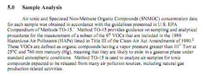
So how did ERG and the TCEQ analyze for carbon disulfide?  They used the correct method, TO-15.

ERG Report

TCEQ Report

And what did Alisa Rich (2) and Dr. Sattler (3) use for their reports?

Dish, Texas Report

FWLN Report

So the wrong method - TO-14 - was used by Alisa Rich and Dr. Sattler to identify the carbon disulfide.  This creates uncertainty on the validity of all the assumptions that were based off the carbon disulfide quantification.

On the other hand, the use of the correct method - TO-15 - reduces the uncertainty and adds to the validity of the results and assumptions made by the TCEQ and ERG in their reports.

Because we cannot know the true value, assumptions are made.  It then becomes necessary for the report writer to show how sound those assumptions are.  Without representative sampling, without QA/QC, and without using the correct analytical method whereby precision and accuracy could be shown, the assumption presented by the FWLN are invalid.

Our assumptions are only as good as our data is sound.

Air Quality in the Barnett Shale - Part 26: That's a lot of n's!


.

Air Quality in the Barnett Shale - Part 24: How confident in that 10.8 ppbv are you?

It has taken me a bit of time to get through the ERG "Interim Ambient Air Monitoring" Report as well as to re-read the Ft. Worth League of Neighborhoods (FWLN) "Recommendations for policy Changes for Gas Drilling Near Schools" report.

There is a lot of data to take in as well as looking at the methodology and conclusions.  I also try not to take things at face value and check the sources of the information (which is why I cite and link my sources).

So here is the issue;  Holy lots-o-dots Batman!  There's a bat-boat load of oil & gas related activity in the Ft. Worth area! (1)

So it is only natural that the public in and around these sites would question if their health and safety is being impacted.  And, when it comes to their children, as in "ensuring the safety of the 80,000 children who attend FWISD schools (2)" the need to be assured becomes elevated.  So what to do...what to do.

I am critical of bad science because it can cause people to do things that are more detrimental to their health then the thing they they were trying to avoid.  The issue in all of this should not be carbon disulfide.  Carbon disulfide is a non-issue and it is dominating the discussion and taking away from a real dialog which should be; What can we do to make oil & gas activity in and around homes and schools safer and reduce its impact on the environment?

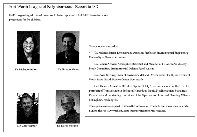
The discussion should be; You want to extract here, then you need to adopt an "Environmentally Systems Drilling Friendly Program" I spoke about in a previous post.  Instead we have a "team of scientists and experts – Dr. Ramon Alvarez, Dr. Melanie Sattler, Dr. DavidSterling, and Carl Weimer – who donated their expertise and time to the League to produce this report (2)" describing a situation of concern that does not exist.

Whether a setback is a prudent idea is not what I am being critical of.  The FWLN report is basing this "one mile setback" on an air dispersion model's finding that carbon disulfide could be found at concentrations over three times the OSHA permissible exposure level (PEL) one mile from an O&G facility. (241 mg/m3 = 78 ppm)

Now reading this, and knowing that a "team of scientists and experts" - two of them Texas University professors - signed off on the findings, one might reasonably conclude; Holy exposure Batman!  The children!

But a closer look at how that number was derived would lead you to a different conclusion; Holy poor science Batman!  That data for carbon disulfide is invalid!

I have tried to present as objective and scientifically based argument as to why this is so in over 24 posts on this topic.  If I have not made my case then either you don't believe me, don't want to believe me, don't want to consider it, or have some other reason to ignore my conclusion as to why the methodology and findings in the Town of Dish Texas and the FWLN reports are wrong.

These blogs are open to anyone who wants to show where my premise, conclusion, or understanding of the science is incorrect, faulty, or wrong.  If I can dish it out (no pun intended) then I sure as better be able to take it.

So it comes down to this.  The FWLN report includes laboratory analysis for carbon disulfide for one single sample:

With the carbon disulfide concentration as:

So the air dispersion model generating Plot 1:

...was based on the analytical report shown above:

And if for no other reason than that - the results of the model and the conclusion for Plot 1 is invalid.  One sample cannot be used to test the null hypothesis that there is a relationship between the ambient air concentration at one location (SUMMA canister for 300 McNaughton Ln.)  and the expected ambient air concentration at another point (one mile out in Plot 1).

One sample is not representative of the air at that location.  Here is what EPA has to say about samples:

Representative: “a sample of a universe or whole (e.g., waste pile, lagoon, ground water) which can be expected to exhibit the average properties of the universe or whole."

Inferences about the population are made from samples selected from the population. For example, the sample mean (or average) is a consistent estimator of the population mean. In general, estimates made from samples tend to more closely approximate the true population parameter as the number of samples increases. The precision of these inferences depends on the theoretical sampling distribution of the statistic that would occur if the sampling process were repeated over and over using the same sampling design and number of samples.

This then leads to:

[a]fter a sample of a certain size, shape, and orientation is obtained in the field (as the primary sample), it is handled, transported, and prepared for analysis. At each stage, changes can occur in the sample (such as the gain or loss of constituents, changes in the particle size distribution, etc.). These changes accumulate as errors throughout the sampling process such that measurements made on relatively small analytical samples (often less than 1 gram) may no longer “represent” the population of interest.  Because sampling and analysis results may be relied upon to make decisions about a waste or media, it is important to understand the sources of the errors introduced at each stage of sampling samples and take steps to minimize or control those errors. In doing so, samples will be sufficiently “representative” of the population from which they are obtained.

When scientists make statements regrading their observations, the concept of precision and bias come into play:

• Precision is a measurement of the closeness of agreement between repeated measurements. 
• Bias is the systematic or consistent over- or underestimation of the true value

Precision is the ability to get the same - or very close - result each and every time you collect or analyze the sample.  Bias, on the other hand, results from a number of problems inherent in sampling and analysis. 

Sampling Bias: 

• Bias can be introduced in the field and the laboratory through the improper selection and use of devices for sampling and subsampling. Bias related to sampling tools can be minimized by ensuring all of the material of interest for the study is accessible by the sampling tool.

• Bias can be introduced through improper design of the sampling plan. Improper sampling design can cause parts of the population of interest to be over- or under-sampled, thereby causing the estimated values to be systematically shifted away from the true values. Bias related to sampling design can be minimized by ensuring the sampling protocol is impartial so there is an equal chance for each part of the waste to be included in the sample over both the spatial and temporal boundaries defined for the study. 

• Bias can be introduced in sampling due to the loss or addition of contaminants during sampling and sample handling. This bias can be controlled using sampling devices made of materials that do not sorb or leach constituents of concern, and by use of careful decontamination and sample handling procedures. For example, agitation or homogenization of samples can cause a loss of volatile constituents, thereby indicating a concentration of volatiles lower than the true value. Proper decontamination of sampling equipment between sample locations or the use of disposable devices, and the use of appropriate sample containers and 

Analytical Bias:

• Analytical (or measurement) bias is a systematic error caused by instrument contamination, calibration drift, or by numerous other causes, such as extraction inefficiency by the solvent, matrix effect, and losses during shipping and handling.

Statistical Bias:

• When the assumptions made about the sampling distribution are not consistent with the underlying population distribution, or
• When the statistical estimator itself is biased.

Because bias is always in play, the number of samples collected (replicates) and the dates/areas (representative) is increased to minimize the impact of these issues.

So how confident in the number 10.8 ppbv is the report's "team of scientists and experts?" How sure are they that 10.8 ppbv represents the true value of the air at that sample point?  I mean. look at all the potential errors that could have impacted it.  Shouldn't at least a duplicate sample have also been collected and analyzed?

It was that one single value that was used to determine the concentration of 78 ppm determined by the model to be in the plume:

Plume extends 1 mile from the source in this graphic. Full extent of plume was in excess of 2 miles. Plot 1 multiples were up to 1000 times the short term health benchmark for carbon disulfide.

How confident would (could) any reputable scientist be if one - and only one - sample - was used in their published research?

For that reason alone, Plot 1 is not valid.

Now, couple that with this:

 Notice that "N" in the very last column?  That's a note from the laboratory:

What the lab is saying is that all the statistical stuff they do - precision & accuracy - was not performed on this sample.  How confident are they in the number 10.8 ppbv?

So there you have it.  Plot 1 was developed using one sample and analyzed on an instrument that was not calibrated for carbon disulfide.

Holy bias Batman!  Plot 1 values are not statistically valid!


Yes Robin, that's what I have been trying to say all along.  The whole enchilada is an example of bad methodology, sampling, and analysis - and the results and conclusion are invalid.


Next post: Air Quality in the Barnett Shale - Part 25: What a statistically valid report looks like.


.

Air Quality in the Barnett Shale - Part 23: Fort Worth League of Neighborhoods Report to FWISD

I received a PDF of a photocopy of a report, dated February 2011, dealing with "Recommendations for Policy Changes for Gas Drilling Near Schools."

As you can see, it brings forth a concern regarding carbon disulfide and uses language that completely disregards the concept of dose, which if you have been reading all 20-something of these posts, was the original issue that started me on this topic.

Okay...so again with the carbon disulfide!  What does this report have to say about that chemical?  Reading... reading.... oh...you have got to be kidding me.  Well no wonder! Seems the same sampling method, the same analytical method, the same premise, the same model assumptions, the same poor science was involved in putting this report together.

It's Dr. Sattler's modeling work!  The same methodology and the same premise was used to produce these setback findings as was performed previously for Alisa Rich.  The same faulty logic that she was raked over the coals for in her December Deposition.  The same methodology I have been writing about in this blog as a way to explain why it is not just wrong, but demonstrably wrong.

I have whipped that dispersion model horse enough, as well as TICs, dose, sample size, and everything else that factors into why her premise and its resulting data are wrong, so I will focus on another factor that really needs to be considered when looking at her work and the conclusion she allows to be made.

What really aggravates me about this is that she knows her work does not meet intellectually honest or scientifically sound practices.  She was told this by the lawyer in the Deposition.  Even if she disagreed, the prudent thing to have done was double checked his concerns.  That obviously did not take place.
And now she not only puts her stamp of approval on it, she brings in another academic, Dr. David Sterling, Chair of Environmental and Occupational Health at the University of North Texas, Health Science Center.  And with him on board, her work, her model's predictions, this report's conclusion, is given the seal of scientifically soundness and approval:

These professionals agreed to assess the information available and make recommendations to the FWISD which could be incorporated into future leases.

This means that all three of them looked at her work and saw nothing wrong with it.  How can this be?

Okay, so lets look at it strictly from a logical point of view.  Let's assume that her model is correct - that every reason I have wrote about is immaterial or does not apply.  So logically if the following is true:

And the model predicted:

This would mean that the emission rate from the source - an emission rate that remains constant for 8760 hours - must be producing way in excess of 241 mg/m3 if that amount was found at up to one mile from the source.

Now according to the model, under calm conditions - perfect so to speak - the concentration at 1000 meters from the stack right smack dab down the center, is 0.001 g/m3 at 1 g/s.  So using that same ratio of dilution, the stack would be putting out at least 241000 mg/s or 241 grams/s of carbon disulfide.

That's a heck of a lot of carbon disulfide in and around the stack.  In fact, to get that much carbon disulfide at one mile from the stack, the amount of carbon disulfide in the immediate area would be at a lethal concentration.

Here is what ATSDR has to say about carbon disulfide (241 mg/m3 = 78 ppm):

• OSHA PEL (permissible exposure limit) = 20 ppm (averaged over an8-hour work shift); 30 ppm (acceptable ceiling concentration; 100 ppm (30-minute maximum peak)
• NIOSH IDLH (immediately dangerous to life or health) = 500 ppm
• AIHA ERPG-2 (maximum airborne concentration below which it is believed that nearly all persons could be exposed for up to 1 hour without experiencing or developing irreversible or other serious health effects or symptoms that could impair their abilities to take protective action) = 50 ppm
• Inhalation is the major route of exposure to carbon disulfide. The vapors are readily absorbed by the lungs. The odor threshold is approximately 200 to 1,000 times lower than the OSHA PEL-TWA (20 ppm). Odors of pure or commercial grades of carbon disulfide usually provide adequate warning of hazardous concentrations

So what this is saying - and here is where the logic comes in - If the one mile concentration could get up to as high as 78 ppm, the emission rate "E" necessary to produce that potential concentration at that distance must be considerably above 78 ppm.  If the model she predicted 241 mg/m3 is true, then the consistent output at the stack must be far greater than 78 ppm.  Which means that whenever the source is in operation, more than 78 ppm of carbon disulfide is being put into the air.

So if the model she predicts 241 mg/m3 is true, the output - "E" - must be producing carbon disulfide in abundance in order to push that much carbon disulfide down the plume to a distance of one mile.

And if that were true, people living in and around these sites at less than1000 meters would be constantly smelling an odor, and - most significantly - these oil & gas production sites would have a lot of very sick or dead workers.

And that is just not happening.  Do people complain about odors?  Yes, but at Dr. Sattler's calculated emission rate, the smell would be constant and never ending since the odor threshold is between  0.1 and 0.2 ppm. And if the level at one mile is 3 times the PEL, the workers at the source would be experiencing consistent health related problems.

This is not happening because there IS NO carbon disulfide being produced at these sites above an amount that will exceed an ESL, cause long or short term harm, or produce an odor.  Not at one mile nor next to the site.  None...at any distance around the facility.

So once again, to show why:

• Dr. Sattler's premise that you can "back in" a concentration to obtain the emission rate "E" is wrong.
• Dr. Sattler's positive identification of carbon disulfide - using EPA Method TO14 - is wrong.
• Dr. Sattler's quantification of carbon disulfide - identified by the lab as a TIC - is wrong.

And because these three things are wrong, her model's predictions are wrong - not off by a little - but wrong.

And because her model's predictions are wrong, the conclusion of the report - based on carbon disulfide concentrations - is wrong.

Next post: Air Quality in the Barnett Shale - Part 24: How confident in that 33.6 ug/m3 are you?

.

Air Quality in the Barnett Shale - Part 22: Gaussian for one, Gaussian for all

I was driving home from San Antonio so I had a lot of "me" time in the car.  Instead of thinking about non-work related stuff, my brain got busy thinking about the air dispersion model used for the Town of Dish, Texas, and for the "Fort Worth League of Neighborhoods" in their report to the Fort Worth Independent School District.

All of the modeling - modeling based on the science and math behind a Gaussian dispersion - is predicated on assumptions.  Not that there is anything wrong with that, it's just that if the assumption holds true in one part it must also hold true for the rest.

So my mind is mulling this over and over.  The math behind it is daunting, especially for a guy like me, but the premise, now that is something I think I do understand.

So in the Gaussian model, which is what Dr. Sattler uses, the premise is this:

If you know the wind direction, wind speed, stack height, atmospheric conditions, and emission rate, you can estimate the plume shape and concentration of the contaminant exiting the stack at any point within the plume.

It assumes that under fixed conditions for that run - fixed air speed, fixed emission rate, fixed atmospheric conditions, fixed exhaust stack height - the plume will behave in a Gaussian manner, that is, along a fixed center line (wind direction) the plume will behave the same on each side of that line.  What these models are used for is to say, that under the most ideal conditions it would be possible for a receptor so many meters away to be potentially exposed to this much of the contaminant at that stack height and that emission rate.

Since there is nothing we can do about the wind and weather, we can adjust the stack height or adjust the emission rate to decrease the intensity of the plume for that receptor.  The emission rate is often tweaked by adding pollution control devices on the stack or limiting the production the entity can produce.  No business likes to do less production so its mostly pollution control devices that are used - or sometimes - raising the height of the stack.

In order for Dr. Sattler to generate her models, she had to assume a fixed condition as well to plug into the computer model, a model that she says uses the Gaussian formula:

She had wind and atmospheric conditions for the day of sampling, so those could be plugged in.  She could reasonably estimate the stack hight for the compressors.  What she didn't have was the actual emission rate.  So it was her reasoning, that if she had the concentration from some point in the plume, she could back in that data and calculate the emission rate that must have been in place to generate that particular concentration under these known conditions (wind speed, direction, atmospheric, stack height, plume location "y").

Now this is completely reasonable in approach.  However it is only reasonable if you assume Gaussian dispersion was taking place.  The model is for Gaussian dispersion, so to calculate an emission rate "E", Gaussian dispersion must be in place for the sample "C" used to back in to the formula.

Again, there is nothing wrong with this premise, as long as a Gaussian dispersion was in operation when the sample was collected.  In order to back in the concentration "C" to get the emission rate "E", Dr. Sattler had to have assumed Gaussian dispersion was in place, since she used a Gaussian formula to calculate the emission rate "E."

So if Gaussian dispersion was in place, and a Gaussian formula was used to calculate the emission rate "E", then the other premise of the Gaussian model is also in place as well:

That at a given emission rate "E" and a wind speed "U", and atmospheric conditions "S" and a stack height "H", somewhere on either side of that center line at location "y" you will find the contaminant to be at concentration "C."

That's when it hit me.

Nothing else is in play here in these Gaussian models.  The chemical's properties, the impact of other agents, pooling, condensing, degradation, vortexes.. they do not exist for purposes of generating these plume models.  It looks at ideal conditions to generate the modeled plume.  The model predicts maximum distance where a particular concentration of the chemical might reasonably be found.

So to "back in" the actual concentration found in a canister, the assumption must be that nothing but a Gaussian plume was being produced when the contaminant was sampled.

If that were the case, the amount of contaminants found in each canisters would be proportional, since the emission rate was steady as was everything else.  Each canister was exposed to the same wind speed "U", the same wind direction "Center Line", the same atmospheric conditions "S", and the same stack height "H".  So taking the location of the canister "y" and the concentration of the contaminant "C" and backing it in to the formula would give you "E".  That's what Dr. Sattler did because that's what she said she did in her deposition.

And with that calculated emission rate "E" she was then able to model the air for 8760 individual plumes - the number of hours in a year for which she had historical data for "U" and "S."  With that data, the emission rate "E", and the estimated stack height "H" - she was able to plug all of that into the model, and using the Gaussian plume formula, calculate both the maximum distance where the dispersion model's plume would show a concentration above a threshold (she used the ESL) as well as calculate the highest possible concentration the source could theoretically produce to which a receptor (citizen in the Town of Dish) might be exposed to.

And that's just what she did for the report, producing Table 2:

Brilliant!  Except for one little bit of a problem.  If the calculated emission rate "E" was determined by backing in the concentration "C" in to the formula, it would produce a theoretical concentration (which she averaged in columns 2 and 5).  If that holds true, then that same emission rate "E" would also be able to produce the actual concentrations in canisters 1 - 6 shown in Table 1.

If it can produce a theoretical, it should also be able to reproduce the actual - since the emission rate "E" was derived from that particular actual data.

This means that canister with the highest amount of benzene - canister 4 - must have been located in the Gaussian plume at a location "y" where the benzene would theoretically be the highest (closer to the center line) when compared to all the other canisters.  Because canister 4 has the highest benzene - because of location "y" - the model holds that at a constant emission rate "E" for the other contaminants was in play as well.

For canister 4 to produce the highest benzene concentration its location in the plume would also produce the highest concentrations for all the other contaminants. Regardless of what "E" is calculated for each contaminant, that "E" was in effect for each canister at exactly the same rate for the six contaminants being discharged on that sample day.  If any of the parameters fluctuated at any time, that impact was felt by all.  The same with wind speed, wind direction, and atmospheric conditions.  The same with stack height.  Each canister was placed and collected under the exact same conditions.  Each canister had to be in the same plume when Dr. Sattler backed in data to generate that emission rate "E."  The conditions producing the actual amount of contaminants in the six canisters must be the same if Gaussian dispersion was in play.

Unless it wasn't.

And if you look at Table 2, you will clearly see it was not.  So if Gaussian dispersion was not taking place that day, then how can you back in the data to calculate an emission rate from a formula that is based on showing a Gaussian dispersion?  If the emission rate "E" that Dr. Sattler calculated cannot be used to calculate the actual concentrations seen, then how can it be used to calculate a theoretical maximum?

And if you ignore that by explaining it away saying the actual concentrations in the six canisters were impacted by other conditions, then you are admitting that Gaussian dispersion was not in play, therefore an emission rate "E" cannot be calculated since no other variables are considered in the formula.

And if you say the sample was collected over 24 hours and was diluted, well that doesn't affect Gaussian dispersion since all the samples were collected for that same period and would have been similarly diluted.

And if you say the wind conditions changed for each of the canisters throughout the day impacting the concentrations of some of the contaminants getting to the canisters, well then, you are really grasping at straws.  And besides, if that's the case, how do you know what concentration to back in to the model?

There are two equally valid reasons why Dr. Sattler's modeling and the subsequent "averaged concentrations" are incorrect:

1. It is impossible to calculate the exact concentration attached to a particular "y" to back into the model because - in real life - the plume is consistently changing over time.  Gaussian modeling assumes perfect and steady conditions in order to produce a plume.  So "E" can never accurately be calculated by backing in the concentration.
2. The concentrations captured in the six canisters came from multiple sources and not from one source as modeled.  In this case, backing those concentrations into the model will always generate an emission rate "E" that is higher than what it is.  This incorrect "E" will then generate plumes and concentrations that are also too high.

Bottom line is this:

If you assume Gaussian dispersion modeling can reasonably model possible concentrations within a plume....

....and you assume that the formula for ground level concentrations is correct:

....and you agree that the canisters were all under the same wind speed, wind direction, and atmospheric conditions...

....and the emission rate "E" was exactly the same for each of the contaminants detected in each of the six canisters...

....and you accept that the emission rate, along with all the other parameters, plugged into that formula will produce a plume that is Gaussian (see graphic at the beginning)....

....then the plume produced from that calculated emission rate "E" must accurately match the actual concentrations found in the six canisters in and around that modeled plume....

...and if the modeled plume - using to emission rate obtained by backing in the actual concentration - does not reproduce the actual concentration that were used to derive it....

....then either the model is wrong....

...or the samples have been impacted by conditions not considered in a Gaussian model....

...which means that the actual concentration found in the six canisters cannot be used to calculate the emission rate of the source....

....which means the data presented in Table 2 of the report, as well as any other report produced using backed in data to find an emission rate, is incorrect.

Bottom-bottom line.

As it stands now, Dr. Sattler's methodology of "backed in" data cannot be used to calculate an emission rate in order to generate plume data to show modeled average concentration levels and/or determine the proper setback for a source.

Bottom-bottom-bottom line:

You cannot use non-Gaussian data to determine the value needed in a formula that produces a Gaussian model.


Next post: The Fort Worth League of Neighborhoods Report to FWISD - Different place, same drummer


.